


7.9 The Ideal Fermi Gas at T = 0: The Fermi Sea and the Stiffness of Matter#
Notebook overview#
Movement III opens where the degeneracy map of §7.8 pointed: dense and light. Copper’s conduction electrons sat four decades above the classical boundary (\(n\lambda_T^3 = 6.8\times10^3\)), and this notebook builds the state they actually occupy. At absolute zero a classical gas does nothing — zero energy, zero pressure, no objection to being squeezed. A gas of fermions cannot afford such rest: the Pauli principle (§6.20) forbids more than one particle per state (two with spin), so the ground state is not “everything in the lowest level” but a filled sea — every state occupied up to a sharp surface, the Fermi energy, with nothing but empty states above it.
The course’s move is to build the sea literally. We take the particle-in-a-box levels of §7.3, sort them, spin-double them, and stack twenty thousand fermions from the bottom. Two honest phenomena appear on the way to the continuum: the highest occupied energy \(\varepsilon_F(N)\) climbs a staircase (degenerate box shells filling one by one, finite-size shell structure presented as physics rather than noise; its grand descendants organize nuclei and metal clusters), and the energy per particle converges to the continuum \(\tfrac35\varepsilon_F\) from above, the occupied-side cousin of the Weyl surface deficit of §7.3. The continuum machinery then delivers the scales, and for real metals the numbers rearrange one’s intuition: copper’s \(\varepsilon_F = 7.0\) eV means \(T_F = 8.2\times10^4\) K, so room temperature is 0.4% of the Fermi temperature — a metal on a lab bench is, for its electrons, a system at effectively absolute zero, each electron carrying about a hundred times the classical thermal energy as pure Pauli zero-point motion, cruising at \(10^6\) m/s in the coldest possible state.
The centerpiece is what the sea does when squeezed: degeneracy pressure, \(P = \tfrac25 n\varepsilon_F \approx 38\) GPa in copper at \(T = 0\) — the statistical repulsion of §7.8 grown into the stiffness of matter — and the claim is put to laboratory data with nothing fitted: the free-electron bulk modulus \(B = \tfrac23 n\varepsilon_F\) lands within 10% of the measured compressibilities of the alkali metals (potassium to 2%), while sodium’s overshoot and copper’s factor-two shortfall are taught as the model’s honest boundary. A stretch exercise turns stiffness into sound (the Bohm–Staver speed predicts sodium’s 3.0 km/s against the measured 3.2: one hears the exclusion principle in a struck metal bar), and the closing computation locates the movement’s summit in advance: the density at which \(v_F\) reaches \(c\) sits exactly at white-dwarf core densities, where the pressure law bends and stars begin to lose the argument with gravity. That cliff belongs to §7.11; this notebook walks to its edge. Everything finite-temperature — \(\mu(T)\), the Sommerfeld corrections, the linear heat capacity, Pauli paramagnetism — is deliberately deferred to §7.10.
Conventions (this notebook). The spin factor 2 is included throughout (and the literal filling spin-doubles the level list before slicing — doubling after silently rescales every energy by \(2^{2/3}\)). Box-model results are labelled finite-size, continuum results continuum. All data comparisons run in SI with CODATA constants in Setup; conduction-electron densities and measured bulk moduli follow Ashcroft & Mermin (Tables 1.1 and 2.1 lineage), with the free-electron counts \(Z = 1\) for the alkalis and copper’s single 4s electron.
How to read the checks. Each exercise closes with a
validatecall against an independent fact: the DOS integral inverted back to \(N\) at eight digits; the literal filling’s \(E/(N\varepsilon_F)\) marching \(0.638 \to 0.620 \to 0.609\) onto the continuum \(\tfrac35\); copper’s \(\varepsilon_F = 7.03\) eV; the \(2^{-2/3}\) volume scaling and a finite-difference check of \(P = -\partial E/\partial V\); the alkali modulus ratios (\(1.02\), \(0.91\), \(0.97\)) against handbook data; Bohm–Staver’s \(3011\) m/s for sodium; and the relativistic threshold \(5.87\times10^{35}\) m⁻³ bracketed by white-dwarf densities. A ✓ is strong evidence; a ✗ is a prompt to locate the discrepancy.Scope. The ideal Fermi gas at exactly \(T = 0\). The warm corrections are §7.10; the relativistic gas and the Chandrasekhar mass are §7.11 (only the threshold is located here); the sea meeting a lattice is §7.12; degenerate doping returns in §7.13. Interacting electrons, screening, and Fermi-liquid theory are named horizons (Volume VIII territory). See Ashcroft & Mermin, Solid State Physics (Ch. 2); Pathria & Beale (Ch. 8); Kittel; Bohm & Staver (1951). Cross-reference §6.20 (Pauli, the sea’s foundation), §7.7 (the step), §7.8 (the degeneracy map and the fermionic virial), §7.3 (the DOS, the counting, the Weyl deficit).
Theory in brief#
The Fermi sea#
At \(T = 0\) the Fermi–Dirac step of §7.7 is exact: every state below \(\mu\) occupied, every state above empty. The ground state of \(N\) fermions is a filled sea, and its surface follows from counting with the density of states of §7.3 (spin factor 2 included):
with \(T_F = \varepsilon_F/k_B\) and \(v_F = \hbar k_F/m\). In \(k\)-space the occupied states fill the Fermi sphere of radius \(k_F\); its boundary, the Fermi surface, is the single concept that organizes all of metal physics — perfectly spherical here, reshaped by a lattice in §7.12.
Filling the sea literally#
The course’s standing move: before trusting the integral, do the count.
and two honest pieces of physics appear. The highest occupied energy \(\varepsilon_F(N)\) climbs a staircase: box shells are degenerate, and each fills completely before the next opens — finite-size shell structure, the tabletop cousin of nuclear magic numbers and the abundance spikes of metal clusters. And the energy per particle approaches the continuum from above, \(E/(N\varepsilon_F) = 0.638, 0.620, 0.609\) at \(N = 10^2, 10^3, 2\times10^4\): the excess is the surface (Weyl) correction of §7.3, returning on the occupied side of the ledger.
The 3/5 and the scales of real metals#
In the continuum the mean kinetic energy per fermion is
and the numbers for real metals deserve slow reading. Copper: \(\varepsilon_F = 7.03\) eV, \(T_F = 8.16\times10^4\) K, \(v_F = 1.57\times10^6\) m/s. Sodium through cesium: \(3.24\) down to \(1.59\) eV. Two consequences. First, \(T_{\text{room}}/T_F = 0.4\)–\(1.6\%\): a metal is always in the deep quantum regime — the \(n\lambda^3 = 6.8\times10^3\) of §7.8 said the same thing from the other side — so this notebook’s \(T = 0\) idealization is accurate to parts in a thousand, and the entire job of §7.10 is the small, Sommerfeld-shaped remainder. Second, each electron carries \(\tfrac35\times7\) eV \(\approx 4\) eV of kinetic energy, roughly a hundred times the classical \(\tfrac32 k_BT\) at room temperature, as pure Pauli zero-point motion: the coldest copper hums at a million metres per second.
Degeneracy pressure: the stiffness of matter#
At fixed \(N\) the total energy scales as \(E = \tfrac35 N\varepsilon_F \propto V^{-2/3}\), so the sea pushes:
pressure at absolute zero, with no interactions and no temperature — the grown-up form of the fermionic virial excess of §7.8. For copper’s electron gas: \(38\) GPa, four hundred thousand atmospheres of outward Pauli push, balanced in the real metal by the electron–ion attraction. This is why ordinary matter resists compression: to shrink the box, the sea must climb its own ladder.
The bulk moduli of real metals: the data jewel#
Differentiating once more gives a zero-parameter prediction from the electron density alone:
Against the handbook: potassium \(3.2\) predicted vs \(3.1\) GPa measured (ratio \(1.02\)), cesium \(0.97\), rubidium \(0.91\) — the alkalis, one loosely bound s-electron over a closed shell and the free-electron poster children, land within 10% with nothing fitted. Sodium overshoots (\(1.46\)) and copper falls short by two (\(0.46\)): the electron–ion softening, the d-band, and the lattice do real work the free gas cannot. A model validated including its boundary — the course’s standing epistemic standard.
The Bohm–Staver sound speed#
Sound in a metal is ions (mass \(M\), valence \(Z\)) oscillating against the electron gas’s spring. At the jellium level the compressibility of the sea sets the restoring force and the ions supply the inertia, and the assembly gives
the Bohm–Staver relation. Predictions with no parameters: sodium \(3011\) m/s against the measured \(\sim3200\); potassium \(1867\) against \(\sim2000\) — 5–7%. The longitudinal ring of a struck metal bar is, to leading order, the Fermi velocity times a mass ratio: one hears the exclusion principle. (Its proper home, the electron–phonon problem, is named and left outward; Ashcroft & Mermin, Solid State Physics, Ch. 26, carries the derivation out in full.)
The edge of the cliff#
\(v_F = \hbar(3\pi^2n)^{1/3}/m_e\) grows with density, and formally reaches \(c\) at
where the kinematics must turn relativistic: \(\varepsilon(k)\) softens from \(\hbar^2k^2/2m\) toward \(\hbar ck\), and the pressure law from \(n^{5/3}\) toward \(n^{4/3}\). Locate the threshold physically: a white dwarf’s core at \(\rho = 10^9\)–\(10^{10}\) kg/m³ (electron density \(n_e = \rho/2u\) for carbon/oxygen composition) brackets \(n_{\text{rel}}\) — the stellar corpses of §7.11 live exactly where the stiffness law bends, and on that bend hangs a maximum mass. The cliff is located; §7.11 walks off it.
Setup#
Data and constants only: the CODATA values, the conduction-electron densities of five metals, and the measured bulk moduli they will be judged against. Every object this notebook is about — the four Fermi scales, the literal filling of the sea, the degeneracy pressure, the free-electron bulk modulus, the Bohm–Staver sound speed — you build in the exercise where it is earned.
The Setup below holds this notebook’s data and instruments — nothing you are asked to build. It is collapsed so the building stays yours; expand it whenever you want the details.
Exercise 1 — The sea from the step#
The \(T = 0\) Fermi function fills a sphere in \(k\)-space, and four scales fall out of its radius. Cite Eq. 726.
Take the \(T \to 0\) limit of the \(n_F\) of §7.7 and state the filled-sea ground state: occupation 1 below \(\varepsilon_F\), 0 above.
Integrate the §7.3 density of states (spin 2) to \(N\) and invert: \(\varepsilon_F = (\hbar^2/2m)(3\pi^2n)^{2/3}\), with \(k_F\), \(T_F\), \(v_F\) defined.
Write
fermi_scales(n, m=M_ELECTRON), returning the four scales you just derived —{'eps_F', 'k_F', 'T_F', 'v_F'}in SI — for a conduction-electron density \(n\). Every later exercise of this notebook is built on it.Verify the inversion numerically with
scipy.integrate.quad: the DOS integral up to the derived \(\varepsilon_F\) returns the density to at least eight digits (copper’s numbers, SI).Name the Fermi surface (prose): the sphere’s boundary in \(k\)-space, the single organizing concept of metal physics — here perfectly spherical, in §7.12 reshaped by a lattice.
copper: ε_F = 7.0328 eV,  k_F = 1.3586e+10 1/m
DOS integral to ε_F: n = 8.470000e+28 1/m^3   (input 8.470000e+28)
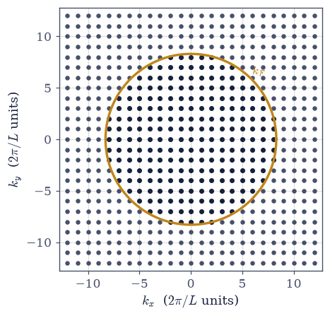
Fig. 653 The Fermi sea in \(k\)-space: a \(k_z = 0\) slice through the filled sphere. Each dot is one allowed momentum state of a periodic box (an integer lattice in units of \(2\pi/L\), two electrons per point with spin); the ground state occupies every state inside the radius \(k_F\) (dark) and none outside (grey) — not because the outer states cost prohibitively much, but because Pauli forbids doubling up anywhere inside. The boundary circle is this slice of the Fermi surface, the single organizing concept of metal physics: everything a metal does thermally or electrically happens within a \(k_BT\)-thin skin of it (Exercise 3 shows that skin is 0.4% deep at room temperature), while the interior is frozen solid by exclusion. Here the surface is a perfect sphere; the lattice of §7.12 will dent and gap it.#
Validation 1#
✓  the Fermi sea: the DOS integral inverted to ε_F returns the density   [got 8.47e+28 vs expected 8.47e+28 (rtol=1e-08, atol=1e-09)]
✓  the closed form ε_F = (ħ²/2m)(3π²n)^(2/3), assembled independently   [got 7.03276 vs expected 7.03276 (rtol=1e-12, atol=1e-09)]
True
Exercise 2 — Filling the sea, literally#
Twenty thousand fermions, stacked by hand — with shell structure and the \(\tfrac35\) emerging from a sorted list. The ordering carries a trap worth stating before it is sprung: the spin doubling must happen before the slice, because doubling afterwards fills \(N\) orbitals instead of \(N/2\) and silently rescales every energy by \(2^{2/3}\), with no crash to flag it. Cite Eq. 727, Eq. 728.
Write
box_levels(nmax): enumerate the positive-integer lattice withnumpy.meshgridup tonmaxper axis, form \(n_x^2 + n_y^2 + n_z^2\) in ground-scale units, flatten, and return itnumpy.sort-ed.Write
fill_sea(levels, N): spin-double withnumpy.repeat(levels, 2), slice the \(N\) lowest, and return the occupied energies together with \(\varepsilon_F(N)\), the highest of them. Write these yourself — the implementation is the lesson.Use them to record \(\varepsilon_F(N)\) and \(E(N)/N\) up to \(N = 2\times10^4\), checking the grid adequacy max(occupied) \(\ll\) nmax².
Confirm \(E/(N\varepsilon_F) = 0.638, 0.620, 0.609\) at \(N = 10^2, 10^3, 2\times10^4\) — converging on \(\tfrac35\) from above — and identify the excess as the surface (Weyl) deficit of §7.3 on the occupied side.
Plot the \(\varepsilon_F(N)\) staircase and read it (prose): degenerate box shells filling one at a time — finite-size shell structure, the tabletop cousin of nuclear magic numbers and metal-cluster stability.
  N =    100:  ε_F(N) =    29.0   E/(N ε_F) = 0.6379
  N =   1000:  ε_F(N) =   113.0   E/(N ε_F) = 0.6196
  N =  20000:  ε_F(N) =   755.0   E/(N ε_F) = 0.6086
grid adequacy: max occupied / nmax^2 = 0.472   (<< 1: the sea fits)
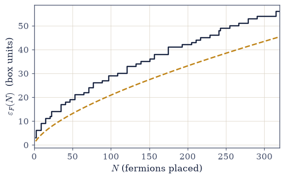
Fig. 654 Finite-size shell structure, presented as physics. The highest occupied energy \(\varepsilon_F(N)\) of the literal filling climbs a staircase: each particle-in-a-box shell (all lattice points sharing \(n_x^2+n_y^2+n_z^2\), times two spins) must fill completely before the surface can move — the wide treads are the big degeneracies. This is the tabletop cousin of the shell structure that gives nuclei their magic numbers and metal clusters their abnormally stable sizes; in the thermodynamic limit the stairs smooth into the continuum \(\varepsilon_F \propto N^{2/3}\) ramp (amber dashed, the sphere-count asymptote), which the box approaches from above: the Weyl surface deficit of §7.3, returning on the occupied side. The step plot draws the physics honestly: a smoothed line would erase exactly what a finite system feels.#
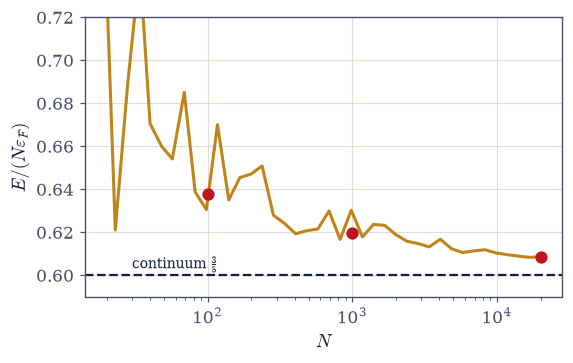
Fig. 655 The continuum, approached from above. The mean energy per particle of the literally filled sea, \(E/(N\varepsilon_F)\), against \(N\) on a log axis: \(0.638 \to 0.620 \to 0.609\) at \(N = 10^2, 10^3, 2\times10^4\), converging on the exact continuum value \(\tfrac35\) (dashed). The excess is the Weyl surface correction of §7.3 read from the occupied side — the box boundary deletes states that the sphere-volume count assumes, so a finite sea sits proportionally deeper below its own surface — and it decays like the slow \(N^{-1/3}\) of a surface-to-volume ratio. Twenty thousand particles still miss the thermodynamic limit by well over a percent: ‘large’ is a matter of surface, not of headcount.#
Validation 2#
✓  the literal filling: E/(N ε_F) = 0.638 → 0.620 → 0.609, marching on the continuum 3/5   [max|Δ| = 0.000442478 (rtol=0.01, atol=1e-09)]
✓  the approach is monotone from above (the Weyl deficit, occupied side) on an adequate grid   [headroom 0.472]
True
Exercise 3 — Metals by the numbers#
Five elements, four scales each — and a room-temperature metal revealed as a zero-temperature system. Cite Eq. 728.
Verify the continuum \(\langle\varepsilon\rangle = \tfrac35\varepsilon_F\) with
scipy.integrate.quadon the DOS moments, then tabulate \(\varepsilon_F\), \(T_F\), \(v_F\) for Cu, Na, K, Rb, Cs from their conduction-electron densities, using thefermi_scalesyou wrote in Exercise 1 (density sources in Setup).Confirm the verified values (Cu: \(7.03\) eV, \(8.16\times10^4\) K, \(1.57\times10^6\) m/s; Na \(3.24\), K \(2.12\), Rb \(1.86\), Cs \(1.59\) eV) and compute \(T_{\text{room}}/T_F\) for each.
Compare the mean kinetic energy \(\tfrac35\varepsilon_F\) against the classical \(\tfrac32k_BT\) at 300 K (\(\sim\)100×), and state what it is: Pauli zero-point motion.
Draw the license (prose): metals are always deeply degenerate (the \(n\lambda^3 = 6.8\times10^3\) of §7.8 re-read), the \(T = 0\) idealization is accurate to \(\sim10^{-3}\), and the task of §7.10 is precisely the small, Sommerfeld-shaped rest.
⟨ε⟩/ε_F by quad: 0.6000000000   (continuum 3/5 = 0.6)

metal   n (1/m^3)     ε_F (eV)   T_F (K)      v_F (m/s)    T_room/T_F
  Cu   8.47e+28     7.03   8.161e+04   1.573e+06   0.37%
  Na   2.65e+28     3.24   3.761e+04   1.068e+06   0.80%
  K    1.40e+28     2.12   2.458e+04   8.632e+05   1.22%
  Rb   1.15e+28     1.86   2.156e+04   8.084e+05   1.39%
  Cs   9.10e+27     1.59   1.844e+04   7.477e+05   1.63%

(3/5)ε_F / (3/2)k_B·300K for copper: 109×
Validation 3#
✓  the continuum mean: ⟨ε⟩ = (3/5)ε_F by quadrature on the DOS moments   [got 0.6 vs expected 0.6 (rtol=1e-10, atol=1e-09)]
✓  the scales of real metals: ε_F from the electron density alone   [max|Δ| = 0.00276129 (rtol=0.01, atol=1e-09)]
✓  T_room/T_F ≤ 1.6% for every metal: a lab-bench metal is an absolute-zero system   [Cu: 0.37%]
True
Exercise 4 — Degeneracy pressure#
A gas at absolute zero that pushes with four hundred thousand atmospheres. Cite Eq. 729.
Derive \(P = \tfrac23 E/V = \tfrac25 n\varepsilon_F\) from \(E \propto V^{-2/3}\) at fixed \(N\).
Write
degeneracy_pressure(n, m=M_ELECTRON), returning \(P = \tfrac25 n\varepsilon_F\) in pascals on top of thefermi_scalesyou wrote in Exercise 1.Verify the \(V\)-scaling by the literal filling (the occupation list is volume-independent, so the box ratio is exact) and, independently, check \(P = -\partial E/\partial V\) against a central finite difference of the continuum \(E(V)\) at copper’s density.
Evaluate \(P\) for copper (\(38\) GPa at \(T = 0\), about \(4\times10^5\) atm) and state what balances it in a real metal (the electron–ion attraction).
Connect backward and forward (prose): this is the statistical repulsion of §7.8 at full strength — the fermionic virial’s \(+n\lambda^3/2^{5/2}\) grown into the incompressibility of matter — and the same push will hold up a dead star in §7.11.
literal filling: E(2V)/E(V) = 0.6299605249   (2^(−2/3) = 0.6299605249)
P by finite difference of E(V): 38.1751 GPa
P = (2/5) n ε_F:                38.1751 GPa

copper's degeneracy pressure: 38.2 GPa ≈ 3.77e+05 atm
Validation 4#
✓  degeneracy pressure: Pauli's 38 GPa push in copper, and the exact V^(−2/3) scaling   [max|Δ| = 0.0249449 (rtol=0.01, atol=1e-09)]
✓  P = −∂E/∂V by central differences meets (2/5)nε_F: the exponent earned, not assumed   [got 3.81751e+10 vs expected 3.81751e+10 (rtol=1e-06, atol=1e-09)]
True
Exercise 5 — The stiffness of real metals: a zero-parameter test#
The bulk modulus from the electron density alone, against the handbook — triumph and honest failure in one bar chart. Cite Eq. 730.
Derive \(B = \tfrac53 P = \tfrac23 n\varepsilon_F \propto n^{5/3}\).
Write
bulk_modulus(n, m=M_ELECTRON), returning \(B = \tfrac53 P\) in pascals on top of thedegeneracy_pressureyou wrote in Exercise 4.Compute \(B\) for Na, K, Rb, Cs, Cu and compare against the measured values (\(6.3, 3.1, 2.5, 1.6, 137\) GPa; Ashcroft & Mermin lineage, stated in Setup).
Confirm the ratios (\(1.46, 1.02, 0.91, 0.97, 0.46\)) and plot the free-vs-measured bar chart.
Read the pattern (prose): the alkalis, with one nearly free s-electron, agree to \(\sim\)10% with nothing fitted; sodium’s excess and copper’s factor-two shortfall mark where the free gas ends (electron–ion softening; the d-band and lattice) — a model validated including its boundary, the course’s standing epistemic standard.
metal   B_free (GPa)   B_measured (GPa)   ratio
  Na        9.17             6.3          1.46
  K         3.17             3.1          1.02
  Rb        2.28             2.5          0.91
  Cs        1.54             1.6          0.97
  Cu       63.63           137.0          0.46
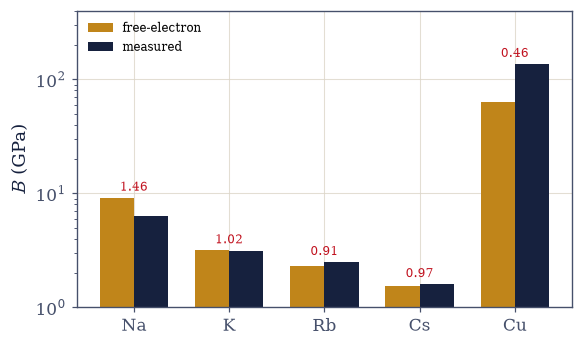
Fig. 656 A zero-parameter test of Pauli stiffness. Free-electron bulk moduli \(B = \tfrac23 n\varepsilon_F\) (amber), computed from each metal’s conduction-electron density and nothing else, against the measured moduli (dark; Ashcroft & Mermin lineage), log scale. The alkalis — potassium, rubidium, cesium, the free-electron poster children — agree to \(\sim\)10% (ratios \(1.02, 0.91, 0.97\)): the compressibility of a real metal reproduced from three constants of nature and a density. The instructive failures: sodium overshoots (\(1.46\): the electron–ion system softens in ways jellium omits) and copper falls short by two (\(0.46\): its filled d-band, invisible to the free gas, carries real stiffness; the bands of §7.12 will name it). The stiffness of ordinary matter is, to leading order in its simplest metals, degeneracy pressure’s derivative — counting, differentiated twice.#
Validation 5#
✓  the compressibility of potassium from ε_F alone: a zero-parameter 2% agreement   [got 1.02174 vs expected 1.02 (rtol=0.03, atol=1e-09)]
✓  the full pattern: alkalis within 10%, sodium's overshoot, copper's honest factor two   [max|Δ| = 0.00445673 (rtol=0.03, atol=1e-09)]
True
Exercise 6 — The sound of Pauli#
The Bohm–Staver relation: a metal’s sound speed from its Fermi velocity and a mass ratio. Cite Eq. 731.
Assemble \(v_s = v_F\sqrt{Zm_e/3M}\) from the jellium picture — ions of mass \(M\) riding the electron gas’s spring, the derivation sketched at the compressibility level (its named home is the electron–phonon problem).
Write
bohm_staver(n, Z, M_ion), returning \(v_s\) in m/s from thefermi_scalesyou wrote in Exercise 1.Predict \(v_s\) for Na and K (valence 1, ion masses from the atomic weights).
Confirm \(3011\) m/s vs measured \(\sim3200\) (Na) and \(1867\) vs \(\sim2000\) (K) — 5–7% with no parameters.
Reflect (prose): the longitudinal ring of a struck sodium bar is, to leading order, the exclusion principle times \(\sqrt{m_e/M}\) — quantum statistics audible across a room.
Bohm–Staver:  Na 3011 m/s   (measured ~3200)
              K  1867 m/s   (measured ~2000)
agreements: 94.1% and 93.3% of measured — no parameters
Validation 6#
✓  Bohm–Staver: the sound of the exclusion principle in sodium   [got 3011.4 vs expected 3011 (rtol=0.02, atol=1e-09)]
✓  and in potassium: 5–7% of measurement with no parameters   [got 1866.74 vs expected 1867 (rtol=0.02, atol=1e-09)]
True
Exercise 7 — The edge of the cliff#
Where the Fermi velocity meets the speed of light — and which objects in the universe live there. Cite Eq. 732.
Set \(\hbar k_F/m_e = c\) and solve: \(n_{\text{rel}} = (m_ec/\hbar)^3/3\pi^2\); evaluate.
Convert white-dwarf central densities \(\rho = 10^9\) and \(10^{10}\) kg/m³ to electron densities (\(n_e = \rho/2u\) for C/O composition) and confirm they bracket \(n_{\text{rel}}\).
State the consequence (one derivation step + prose): relativistic kinematics softens \(\varepsilon(k)\) from \(k^2/2m\) toward \(ck\), hence \(P\) from \(n^{5/3}\) toward \(n^{4/3}\) — the stiffness law bends exactly where the dead stars live.
Pose the question of §7.11 (prose): a star held up by a pressure that softens under compression is a star that can lose — above what mass does gravity win?
n_rel = (m_e c/ħ)^3 / 3π² = 5.865e+35 1/m^3
(copper, for scale: 8.5e+28 — seven decades below)

white-dwarf cores: n_e(ρ=1e9) = 3.01e+35  → n_e/n_rel = 0.51
                   n_e(ρ=1e10) = 3.01e+36  → n_e/n_rel = 5.13

ε ~ k²/2m → P ∝ n^(5/3)   |   ε ~ ħck → P ∝ n^(4/3): the law bends at n_rel
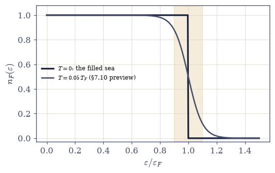
Fig. 657 The state this notebook built, and the sliver the next one warms. The occupation of the Fermi sea at \(T = 0\) (dark): a perfect step at \(\varepsilon_F\) — every state below filled, every state above empty, the idealization that Exercise 3 licensed at the parts-per-thousand level for laboratory metals. Greyed: the same sea at \(T = 0.05\,T_F\), an exaggerated preview of §7.10 — thermal smearing touches only a \(k_BT\)-wide shell at the surface (the shaded sliver), because deeper electrons have no empty states within thermal reach. Everything a metal does at room temperature — its heat capacity, its magnetism, its transport — happens in that sliver, which is why the corrections of §7.10 are small, linear in \(T\), and Sommerfeld-shaped.#
Validation 7#
✓  the relativistic threshold: v_F = c at (m_e c/ħ)³/3π²   [got 5.86516e+35 vs expected 5.87e+35 (rtol=0.01, atol=1e-09)]
✓  white-dwarf core densities bracket the threshold: the dead stars live on the bend   [ratios 0.51 and 5.13]
True
Exercise 8 — The stiffness of the world#
The classical gas met absolute zero by giving up — no energy, no pressure, no objection to being squeezed. The fermion gas met it by building a sea. Everything in this notebook flowed from that refusal: energies of electron-volts where classical physics offered hundredths, a room-temperature wire that is effectively at absolute zero, thirty-eight gigapascals of outward push in resting copper, the measured stiffness of potassium reproduced from its electron density and three constants of nature, and the ring of a metal bar carrying the exclusion principle to the ear. Volume V’s gases pushed on walls because they were hot; this one pushes because it is full.
It is worth sitting with the strangeness. Nothing is hot, nothing attracts, nothing repels — and yet the gas pushes hard enough to hold up stars, because arithmetic forbids it to rest. Degeneracy pressure may be the purest force in physics: a pressure made of counting.
The next notebook warms the sea by its actual 0.4% (§7.10: the Sommerfeld corrections, the linear heat capacity, Pauli’s paramagnetism), and the one after follows the pressure to its greatest stage — a dying star weighing Pauli against gravity (§7.11). Then the sea meets a lattice (§7.12), and the movement discovers why some seas cannot flow at all.
Notebook summary#
Movement III opens with the ground state of dense, light matter — built by counting, checked against handbooks.
The Fermi sea Eq. 726: the \(T = 0\) step fills the sphere \(|k| \le k_F\); \(\varepsilon_F = (\hbar^2/2m)(3\pi^2n)^{2/3}\) inverted and verified by quadrature; the Fermi surface named as metal physics’ organizing concept.
The sea, filled literally Eq. 727: sorted box levels, spin-doubled before slicing (the \(2^{2/3}\) trap stated); the \(\varepsilon_F(N)\) shell staircase taught as finite-size physics (nuclear magic numbers’ tabletop cousin); \(E/(N\varepsilon_F) = 0.638 \to 0.620 \to 0.609\), converging on \(\tfrac35\) from above — the Weyl deficit, occupied side.
Metals by the numbers Eq. 728: Cu \(\varepsilon_F = 7.03\) eV, \(T_F = 8.2 \times10^4\) K, \(v_F = 1.6\times10^6\) m/s; \(T_{\text{room}}/T_F = 0.4\)–\(1.6\%\) — metals live at absolute zero, each electron carrying \(\sim\)100× the classical thermal energy as Pauli zero-point motion. The license of §7.10, written.
Degeneracy pressure Eq. 729: \(P = \tfrac25 n\varepsilon_F = 38\) GPa in copper — the \(V^{-2/3}\) scaling exact in the literal filling and earned by finite differences in the continuum — the virial excess of §7.8 grown into the stiffness of matter.
The data jewel Eq. 730: \(B = \tfrac23 n\varepsilon_F\) against the handbook — K \(1.02\), Rb \(0.91\), Cs \(0.97\) with nothing fitted; Na’s \(1.46\) and Cu’s \(0.46\) taught as the model’s honest boundary (electron–ion softening; the d-band).
The sound of Pauli Eq. 731: \(v_s = v_F\sqrt{Zm_e/3M}\) — sodium \(3011\) m/s vs \(\sim3200\) measured: the exclusion principle, audible.
The cliff, located Eq. 732: \(v_F = c\) at \(n_{\text{rel}} = 5.87\times10^{35}\) m⁻³ — bracketed by white-dwarf core densities (ratios \(0.51\) and \(5.1\)); the pressure law bends from \(n^{5/3}\) to \(n^{4/3}\) exactly where the dead stars live. §7.11 walks off the edge.
A pressure made of counting; next, its thermal corrections, and then its greatest stage.
Outlook#
The sea, warmed by 0.4% (§7.10). \(\mu(T)\), the linear heat capacity, Pauli paramagnetism — the Sommerfeld program, tooled in §7.3.
The pressure’s greatest stage (§7.11). White dwarfs and the Chandrasekhar mass — the relativistic gas developed in full.
The sea meets a lattice (§7.12). Bloch, bands, and why some seas cannot flow; degenerate doping returns in §7.13.
Interacting electrons (screening, Fermi-liquid theory): named horizons, Volume VIII territory.
Cross-reference §6.20 (Pauli, the sea’s foundation), §7.7 (the step), §7.8 (the degeneracy map; the virial embryo), §7.3 (the DOS, the counting, the Weyl deficit — twice reused here).