


2.11 Nonlinear Dynamics and Chaos: When Integrability Fails#
Notebook overview#
§2.10 closed the integrable half of mechanics: when a full set of action variables exists, motion winds forever on invariant tori, and the Outlook admitted the catch — when no separation exists the tori break. This notebook is that horizon, made quantitative. The course has already met chaos three times informally: the driven pendulum’s period-doubling cascade in §1.2, the double pendulum’s positive Lyapunov exponent in §1.3, and the Hénon–Heiles sections of §5.5 (a Volume V notebook that borrows this one’s subject for statistical ends). What none of them did is measure the universal numbers — and universal numbers, it turns out, is exactly what chaos has.
We work in three acts. First the logistic map, the fruit fly of dynamics [May76]: one quadratic formula whose period-doubling cascade converges at the rate \(\delta = 4.669\,201\ldots\), a constant we measure to five digits and then measure again in a completely different map, because Feigenbaum’s discovery [Fei78] is that the constant belongs to the transition, not the equation. Second the kicked rotor, whose stroboscopic standard map [Chi79] shows Hamiltonian chaos the way Volume II should see it: resonance islands widening as \(\sqrt{K}\), the last invariant torus dying at Greene’s \(K_c = 0.9716\) [Gre79], and beyond it deterministic motion that diffuses like a random walk, with a diffusion coefficient we predict. Third the Lorenz system [Lor63], where we measure the largest Lyapunov exponent of a flow two independent ways and reproduce Lorenz’s own beautiful argument — a one-dimensional return map hiding inside a three-dimensional butterfly — that the attractor can contain no stable orbit at all. The standard text for everything here is Strogatz [Str15].
A note on reading the checks in this notebook: a validation compares a result to an expected physical fact. A ✗ does not by itself mean the answer is wrong; it means the output did not match what the check expected, which may be a genuine error, a different-but-valid convention, or too tight a tolerance. Treat a ✗ as a prompt to locate the discrepancy. Passing is strong evidence, not proof.
Theory in brief#
Maps as dynamics. A first-order recursion \(x_{n+1} = f(x_n)\) is the simplest dynamical system there is, and everything this notebook needs already lives in it. Our laboratory specimen is the logistic map
May’s toy model of a population with reproduction rate \(r\) and crowding [May76]. A fixed point \(x^* = f(x^*)\) attracts when \(|f'(x^*)| < 1\) and repels when \(|f'(x^*)| > 1\): perturb by \(\epsilon\) and one step gives \(f(x^* + \epsilon) \approx x^* + f'(x^*)\,\epsilon\), so the derivative is the per-step amplification factor. For Eq. 182 the non-trivial fixed point is \(x^* = 1 - 1/r\) with \(f'(x^*) = 2 - r\): stable for \(1 < r < 3\), and at exactly \(r = 3\) the derivative reaches \(-1\) and the fixed point hands over to a period-2 cycle (a period-doubling bifurcation). The cycle then doubles again at \(r = 1 + \sqrt 6 = 3.449\,49\ldots\), and again, and again, the doublings accumulating at \(r_\infty = 3.569\,95\ldots\) beyond which chaos begins.
Feigenbaum universality. The bifurcation parameters converge geometrically, and their rate is the discovery. Using the superstable parameters \(R_n\) (those where the \(2^n\)-cycle passes through the map’s maximum \(x_c = 1/2\), so the cycle derivative is exactly zero: the numerically cleanest markers of each doubling), the ratios
converge to Feigenbaum’s constant, and the cycle’s distance scale shrinks by \(\alpha = -2.502\,907\ldots\) per doubling. The stunning part, proved by renormalization: \(\delta\) and \(\alpha\) are the same for every map with a quadratic maximum — the logistic map, \(r\sin(\pi x)\), the driven pendulum of §1.2, a dripping faucet, convecting helium. We verify universality the honest way, by measuring \(\delta\) twice in two unrelated maps.
The word universality is the same one statistical mechanics uses, and so is the mechanism. Feigenbaum’s argument is a renormalization in miniature: rescale the map near its maximum, iterate the rescaling, and \(\delta\) and \(\alpha\) fall out as properties of the fixed point the rescaling flows to, which is why every quadratic-maximum map inherits them regardless of its details. The thermodynamic version of exactly that story, where distinct systems share critical exponents because the coarse-graining flow forgets their microscopic differences, is §5.10 and E.3. Constructing the renormalization group is a stated boundary of this course in both places, and it is a boundary here too; the point is only that the two universalities are one idea.
The Lyapunov exponent of a map. Chaos is exponential sensitivity, and for a map the growth rate of an infinitesimal error after \(n\) steps is the product of the per-step derivatives, so its logarithmic average
is the map’s Lyapunov exponent: \(\lambda < 0\) on periodic attractors, \(\lambda = 0\) at each bifurcation (the handover moment where \(|f'| = 1\) around the cycle), \(\lambda > 0\) in chaos. One value is known exactly: at \(r = 4\) the substitution \(x = \sin^2(\pi y / 2)\) conjugates Eq. 182 to the tent map, each step of which doubles \(y\)-errors, so \(\lambda(4) = \ln 2\) — an analytic benchmark for the numerical average.
Hamiltonian chaos: the kicked rotor. Volume II’s own route to chaos starts from §2.10’s action-angle picture. Take the freest system imaginable — a rigid rotor with angle \(\theta\) and (scaled) angular momentum \(p\), no gravity — and kick it impulsively once per period with a torque \(K\sin\theta\). Between kicks \(p\) is constant and \(\theta\) advances by \(p\); integrating across one period gives the standard map [Chi79]
an area-preserving map of the cylinder that is the local model of any Hamiltonian resonance. At \(K = 0\) every orbit lies on a torus \(p = \text{ const}\): §2.10’s integrable picture, stroboscoped. Small \(K\) replaces the resonant torus \(p = 0\) by a pendulum-like island of half-width \(2\sqrt K\) (Chirikov’s resonance-width estimate), while non-resonant tori survive as slightly wavy KAM curves that bar vertical transport: an orbit cannot cross an invariant curve. As \(K\) grows the islands widen, KAM curves die one by one, and the most robust — the torus with golden-mean winding number — dies last, at Greene’s critical \(K_c = 0.971\,635\ldots\) [Gre79]. Beyond \(K_c\) nothing bars the way: \(p\) performs a deterministic random walk, and for large \(K\) the phases \(\theta_n\) decorrelate so effectively that \(\langle p_n^2 \rangle \approx 2 D n\) with the quasilinear coefficient \(D_{\rm ql} = K^2/4\) (the variance of one kick, \(\langle K^2\sin^2\theta \rangle = K^2/2\), accumulated as an uncorrelated walk). Correlations between kicks decorate \(D\) with oscillatory Bessel-function corrections whose leading term is proportional to \(J_2(K)\); we dodge the decoration by measuring at a zero of \(J_2\).
Chaos in a flow: Lorenz. Continuous-time chaos needs three dimensions, and the canonical specimen is Lorenz’s convection model [Lor63]
at the classical parameters \(\sigma = 10\), \(\rho = 28\), \(\beta = 8/3\). Trajectories collapse onto the butterfly-shaped strange attractor and separate on it at the rate given by the largest Lyapunov exponent, \(\lambda_1 \approx 0.9056\) (in inverse Lorenz time units): predictability is lost with a half-life of order \(\ln 2 / \lambda_1 \approx 0.77\) time units, which is the quantitative content of the “butterfly effect”. The measurement tool is Benettin renormalization — run a reference and a companion trajectory, and every interval \(\tau\) record the logarithm of their separation growth and rescale the companion back to distance \(d_0\) along the current separation direction (rescaling before saturation is what keeps the measurement in the linear regime the exponent describes.)
Setup#
Everything runs in dimensionless units: the maps on their natural intervals, the standard map on the cylinder \(\theta \in [0, 2\pi)\), Lorenz in Lorenz’s own time units. Randomness appears only in the choice of ensemble initial conditions for the diffusion experiment and is seeded. Setup holds that seed, the reference values the measurements are checked against (\(\delta\), \(\alpha\), and Lorenz’s \(\lambda_1\)), and the specimen systems themselves — the logistic map Eq. 182 with its derivative, and the Lorenz right-hand side Eq. 186 — transcribed from the theory above, because they are what the problem hands you rather than anything anyone builds. The measuring machinery is not here: you write the attractor-period detector and the bisection that locates a doubling (Exercise 1), the tangent-recursion Newton solver for the superstable ladder (Exercise 2), the Lyapunov average (Exercise 4), the standard-map stepper (Exercise 5), and the Benettin renormalization (Exercise 6).
The Setup below holds this notebook’s data and instruments — nothing you are asked to build. It is collapsed so the building stays yours; expand it whenever you want the details.
Exercise 1 — The logistic laboratory#
Everything begins with Eq. 182 and its fixed points. Setting \(x^* = r x^* (1 - x^*)\) gives \(x^* = 1 - 1/r\), with derivative \(f'(x^*) = 2 - r\); the linearization argument of the theory section says this fixed point holds the population steady only while \(|2 - r| < 1\). Past \(r = 3\) the map settles instead onto the period-2 cycle whose two points are the roots of \(f(f(x)) = x\) that are not fixed points of \(f\), which factor out to
real exactly when \(r \ge 3\): the cycle is born at the bifurcation.
Part a) At \(r = 2.9\), iterate Eq. 182 from \(x_0 = 0.2\)
for \(500\) steps and verify the orbit converges to \(x^* = 1 - 1/2.9\) to
\(|x_{500} - x^*| < 10^{-10}\), and that the measured convergence is
governed by \(f'(x^*) = 2 - r = -0.9\) (compare logistic_prime(x*, 2.9)
to \(-0.9\) at rtol=1e-12). At \(r = 3.2\), verify the same fixed point now
repels (\(|f'(x^*)| > 1\)) and that \(2000\) iterations from \(x_0 = 0.2\)
land on the two-cycle: the final two iterates match \(x_\pm\) above
(numpy.sort then validate.close, rtol=1e-10).
Part b) Draw the cobweb construction at \(r = 2.8\) (spiral into the fixed point), \(r = 3.4\) (the period-2 square), and \(r = 3.9\) (chaotic tangle): plot the parabola \(f(x)\) and the diagonal \(y = x\), then the staircase segments \((x_n, x_n) \to (x_n, x_{n+1}) \to (x_{n+1}, x_{n+1})\) for \(60\) iterations from \(x_0 = 0.2\).
Part c) Write the two pieces that turn “the period doubled somewhere in
here” into a number. First attractor_period(r): iterate past the
transient, then compare the settled orbit with itself shifted by
\(1, 2, 4, \ldots, 32\) steps and return the first shift that reproduces it
to a tolerance, with \(64\) standing for “longer than \(32\), or chaotic”. The
burn-in has to be long — tens of thousands of iterations, not hundreds —
because near a bifurcation the transient decays critically slowly. Then
bisect_doubling(period_from, lo, hi), which bisects on that detector: a
parameter whose period is still period_from moves the lower edge up, a
longer period moves the upper edge down. Write these yourself — the
implementation is the lesson.
Part d) Build the orbit (bifurcation) diagram: for each of \(1400\)
parameters \(r \in [2.8, 4.0]\), iterate a vectorized ensemble \(800\) burn-in
steps and scatter the next \(300\) iterates. Then measure the first two
bifurcation points with your bisect_doubling (period \(1 \to 2\)
between \(r = 2.8\) and \(3.2\); period \(2 \to 4\) between \(3.3\) and \(3.5\)) and
verify them against the exact \(r_1 = 3\) and \(r_2 = 1 + \sqrt 6\)
(rtol=1e-3; the residual is the period-detector’s finite tolerance
fighting critical slowing-down, not the mathematics).
r=2.9: |x_500 - x*| = 3.33e-16, f'(x*) = -0.900000
r=3.2: |f'(x*)| = 1.200 (repels)
2-cycle numeric [0.51304451 0.79945549] vs exact [0.51304451 0.79945549]
✓ at r = 2.9 the orbit converges onto x* = 1 - 1/r [|x_500 - x*| = 3.3e-16]
✓ and the measured stability factor is f'(x*) = 2 - r = -0.9 exactly [got -0.9 vs expected -0.9 (rtol=1e-12, atol=1e-09)]
✓ at r = 3.2 the same fixed point has |f'| > 1: it repels [|f'| = 1.200]
✓ and the orbit lands on the period-2 cycle at its closed-form points x± = ((r+1) ± √((r-3)(r+1)))/(2r) [max|Δ| = 1.11022e-16 (rtol=1e-10, atol=1e-09)]
True
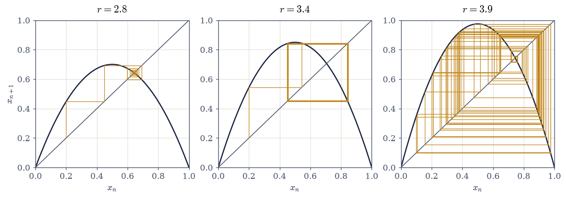
Fig. 171 Cobweb constructions for the logistic map \(x_{n+1}=rx_n(1-x_n)\) at three parameters, each iterated 60 steps from \(x_0=0.2\): at \(r=2.8\) the staircase spirals into the stable fixed point \(x^*=1-1/r\) (the parabola–diagonal crossing); at \(r=3.4\) it settles onto the period-2 square; at \(r=3.9\) it wanders chaotically over the interval. The parabola is \(f(x)\), the diagonal is \(y=x\), and each step reflects the orbit between them.#
measured r1 = 2.999810 (exact 3)
measured r2 = 3.449417 (exact 1+√6 = 3.449490)
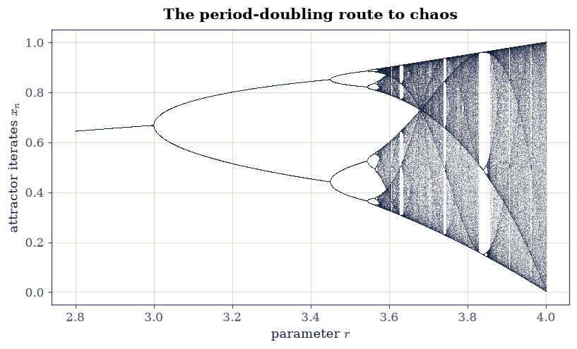
Fig. 172 The orbit (bifurcation) diagram of the logistic map: for each of 1400 parameters \(r\in[2.8,4.0]\) the attractor is sampled by 300 iterates after an 800-step transient. The single branch is the stable fixed point \(1-1/r\); it splits at \(r_1=3\), splits again at \(r_2=1+\sqrt6\approx3.449\), and the doublings accumulate at \(r_\infty\approx3.570\) into the chaotic band, which is punctured by periodic windows (the wide one near \(r\approx3.83\) has period 3).#
✓ the first period-doubling, located by bisection on the attractor period, sits at r1 = 3 [got 2.99981 vs expected 3 (rtol=0.001, atol=1e-09)]
✓ and the second at r2 = 1 + √6 = 3.44949 [got 3.44942 vs expected 3.44949 (rtol=0.001, atol=1e-09)]
True
Exercise 2 — Feigenbaum’s constants, measured#
The doubling cascade of Fig. 172 accumulates geometrically, and Eq. 183 defines the rate. To measure it we need the superstable parameters \(R_n\) to many digits, and the right tool is Newton’s method on the defining condition \(f^{(2^n)}(x_c; R) = x_c\) with \(x_c = 1/2\). Newton needs the derivative of a \(2^n\)-fold composition with respect to \(R\), and the clean way to get it is the tangent recursion: propagate the pair \((x, \partial x / \partial R)\) through the map together,
which is exact forward sensitivity (the same chain-rule idea that propagates error bars, and a baby version of what automatic differentiation does). Seeding matters: each \(R_n\) is predicted from the previous two by the Feigenbaum ratio itself, because a careless seed lets Newton converge onto a different root of \(f^{(2^n)}(x_c) = x_c\) (every shallower superstable parameter is one) and silently wreck the ladder. Two rungs of the ladder are known in closed form and so make its certificate: \(R_0 = 2\), where \(f(1/2) = 1/2\) exactly, and \(R_1 = 1 + \sqrt 5\), where the 2-cycle passes through the maximum.
Part a) Write superstable_params(f, df_dx, df_dr, n_max, guess1, x_c=0.5), which solves \(f^{(2^n)}(x_c; R) = x_c\) for \(R\) by Newton at
every level \(n\): propagate the pair \((x, \partial x / \partial R)\) through
the map by the tangent recursion above rather than finite-differencing a
\(2^n\)-fold composition, and seed each \(R_n\) by geometric extrapolation from
the previous two with the Feigenbaum ratio. Use it to compute
\(R_0, \ldots, R_8\) for the logistic map; alongside logistic_prime you
will need the other partial, \(\partial f / \partial r = x(1 - x)\).
Write this one yourself — the implementation is the lesson.
Part b) Certify the solver on the two closed-form rungs: verify
\(R_0 = 2\) and \(R_1 = 1 + \sqrt 5\) to atol=1e-9.
Part c) Form the ratios \(\delta_n\) of Eq. 183 and verify the
deepest one, \(\delta_7\), agrees with \(\delta = 4.669\,201\,609\) to
rtol=1e-4. Estimate \(R_\infty\) by geometric extrapolation
\(R_\infty \approx R_8 + (R_8 - R_7)/(\delta - 1)\) and plot
\(R_\infty - R_n\) on a log axis: the straight line is the geometric
convergence.
Part d) Measure \(\alpha\): at each \(R_n\) the cycle point nearest the
maximum sits a distance \(d_n = f^{(2^{n-1})}(x_c; R_n) - x_c\) away, and
successive ratios \(d_n / d_{n+1}\) converge to \(\alpha = -2.502\,908\)
(note the sign: the nearest return alternates sides). Verify the deepest
ratio to rtol=1e-3.
R_n : 2.0000000 3.2360680 3.4985617 3.5546409 3.5666674 …
delta_n : 4.70894 4.68077 4.66296 4.66840 4.66895 4.66916 4.66919
alpha_n : -2.5032 -2.5030 -2.5029
R_inf ≈ 3.5699457 (accumulation of the cascade)
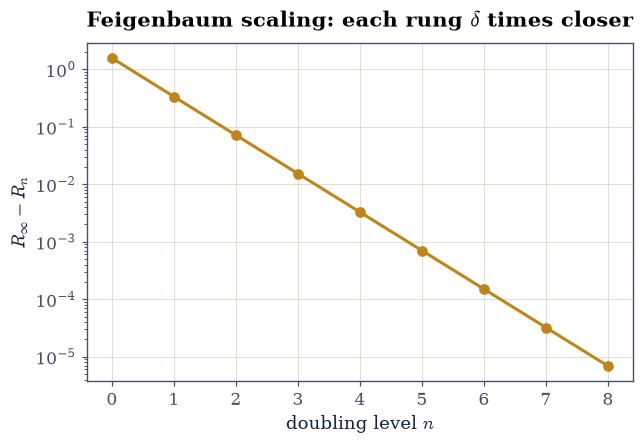
Fig. 173 Geometric convergence of the logistic map’s superstable parameters: the gap \(R_\infty-R_n\) against the doubling level \(n\) on a logarithmic axis, with \(R_\infty\) estimated by geometric extrapolation from the two deepest rungs. The straight-line decay at slope \(-\log_{10}\delta\) per level is Feigenbaum scaling; the fitted ratio gives \(\delta_7=4.66919\) against the exact \(4.669\,201\,609\).#
✓ the solver certifies on the closed-form rung R_0 = 2 [got 2 vs expected 2 (rtol=0, atol=1e-09)]
✓ and on R_1 = 1 + √5, the superstable 2-cycle [got 3.23607 vs expected 3.23607 (rtol=0, atol=1e-09)]
✓ eight doublings deep, the ratio of successive gaps is Feigenbaum's delta = 4.669201609 [got 4.66919 vs expected 4.6692 (rtol=0.0001, atol=1e-09)]
✓ and the nearest-return distances shrink by alpha = -2.502908 per doubling, sign and all [got -2.50292 vs expected -2.50291 (rtol=0.001, atol=1e-09)]
True
Exercise 3 — Universality: a different map, the same constant#
The measurement so far could be a curiosity of the parabola. Feigenbaum’s claim [Fei78] is far stronger: every one-hump map with a quadratic maximum doubles its way to chaos with the same \(\delta\) and \(\alpha\), because near the accumulation point the dynamics is controlled by a renormalization fixed point that has forgotten the original map entirely (the same logic — details washed out under repeated coarse-graining — will return as the explanation of universal critical exponents in §5.10). The honest test is to measure again in a map that shares nothing with the logistic map but the shape of its top: the sine map
transcendental where the logistic map is polynomial, with its cascade living on a completely different parameter interval.
Part a) Reuse the superstable_params you wrote in Exercise 2, now
with \(f = r\sin(\pi x)\),
\(\partial f/\partial x = r\pi\cos(\pi x)\), \(\partial f/\partial r =
\sin(\pi x)\), seeding \(R_1\) at \(0.78\), to compute the sine map’s
\(R_0, \ldots, R_8\). Verify \(R_0 = 1/2\) exactly (where \(r\sin(\pi/2) =
1/2\)) to atol=1e-10, and verify the cascade is not the logistic one:
its \(R_1\) differs from the logistic \(R_1 = 1 + \sqrt 5\) by more than \(2\).
Part b) Form the sine map’s \(\delta_n\) ratios and verify \(\delta_7\)
agrees with the logistic measurement of Exercise 2 to rtol=1e-3: two
maps, two cascades, one constant. Plot the two orbit diagrams one above
the other over their own parameter ranges; the point of the figure is
that they are the same picture stretched differently.
sine R_n : 0.500000 0.777734 0.846382 0.861450 …
sine delta_n: 4.66811 4.66897 4.66915
logistic delta_7 = 4.66919, sine delta_7 = 4.66915
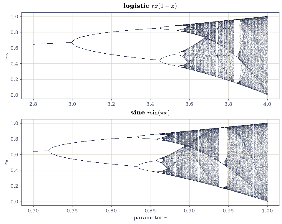
Fig. 174 Orbit diagrams of the logistic map \(rx(1-x)\) over \(r\in[2.8,4.0]\) (top) and the sine map \(r\sin(\pi x)\) over \(r\in[0.7,1.0]\) (bottom), each sampled by 250 post-transient iterates at 1200 parameters. The two maps share no formula, yet the diagrams are the same picture differently stretched: the doubling cascades of both converge with the identical Feigenbaum ratio \(\delta=4.6692\), measured here as 4.66919 (logistic) and 4.66915 (sine).#
✓ the sine map's R_0 = 1/2 exactly (its superstable fixed point) [got 0.5 vs expected 0.5 (rtol=0, atol=1e-10)]
✓ the two cascades live on different parameter intervals: the maps share nothing but the shape of their maximum [|R_1(sine) - R_1(logistic)| = 2.458]
✓ yet their doubling ratios agree: Feigenbaum's constant belongs to the transition, not the equation [got 4.66915 vs expected 4.66919 (rtol=0.001, atol=1e-09)]
True
Exercise 4 — The Lyapunov exponent across the diagram#
The orbit diagram shows where the attractor is; the Lyapunov exponent Eq. 184 says how predictable it is, and laying the two on the same parameter axis turns the bifurcation diagram into an instrument panel. The conjugacy benchmark makes one point of the curve exact: with \(x = \sin^2(\pi y/2)\), the \(r = 4\) logistic map becomes the tent map on \(y\), which stretches every interval by the factor \(2\), so \(\lambda(4) = \ln 2\) precisely.
Part a) Write lyapunov_logistic(r_values, n_iter=20000, burn=1000),
which evaluates Eq. 184 for a whole array of parameters at once:
carry every parameter’s orbit simultaneously as one NumPy array, discard
the burn-in, then accumulate the running mean of \(\ln|f'(x_k)|\) over the
remaining iterations. Guard the logarithm — an orbit landing exactly on
\(x = 1/2\) sends \(|f'|\) to zero, and clipping the argument from below
handles that measure-zero event without biasing the average.
Write this one yourself — the implementation is the lesson.
Part b) Compute \(\lambda(r)\) with it on the \(1400\) parameters of Exercise 1’s grid (\(20\,000\) averaging iterations after a \(1000\)-step transient), and plot it beneath the orbit diagram with the shared \(r\) axis and a zero line.
Part c) Verify the three signatures: (i) the exact benchmark
\(\lambda(4) = \ln 2\) at rtol=1e-3 (with \(2\times10^5\) iterations for
the single-point average); (ii) \(\lambda = 0\) at the bifurcation \(r = 3\)
to atol=2e-3 (the handover moment: the cycle is marginally stable);
(iii) deep in the period-3 window, \(\lambda(3.835) < -0.25\) — order
inside chaos, exactly where Fig. 172 shows the
clear vertical band.
Part d) Measure how much of the chaotic regime is actually chaotic: the fraction of the \(400\)-point grid on \([3.57, 4.0]\) with \(\lambda > 0\), which should land between \(0.85\) and \(0.97\) — the windows puncture the chaos everywhere (Fig. 175 shows them as downward spikes), but they puncture it on a small fraction of parameters.
lambda(4) = 0.693145 vs ln 2 = 0.693147
lambda(3) = -0.00004 (bifurcation: marginal)
lambda(3.835) = -0.3097 (period-3 window)
chaotic fraction of [3.57, 4]: 0.907
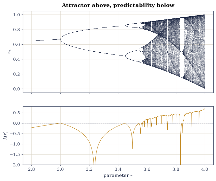
Fig. 175 The instrument panel of the logistic map: the orbit diagram (top) and the Lyapunov exponent \(\lambda(r)\), the orbit-averaged \(\ln|f'|\) (bottom), on the shared parameter axis, with the dashed line at \(\lambda=0\). Every period-doubling touches \(\lambda=0\) from below, chaos is the region \(\lambda>0\) beyond \(r_\infty\approx3.570\), the periodic windows plunge \(\lambda\) negative again (the period-3 window near \(r=3.83\) most visibly), and at \(r=4\) the exponent reaches its exact value \(\ln 2\).#
✓ the exact benchmark: at r = 4 the tent-map conjugacy fixes lambda = ln 2 [got 0.693145 vs expected 0.693147 (rtol=0.001, atol=1e-09)]
✓ at the r = 3 bifurcation the exponent is zero: marginal stability at the handover [lambda(3) = -3.9e-05]
✓ deep in the period-3 window the exponent is decisively negative: order inside chaos [lambda(3.835) = -0.310]
✓ chaos beyond r_inf is punctured by periodic windows on a small but non-zero fraction of parameters [fraction = 0.907]
True
Exercise 5 — The kicked rotor: tori die one by one#
Now the Hamiltonian act. The kicked rotor is the cleanest bridge from §2.10: a free rotor is an action-angle system (its momentum is the action, its angle advances uniformly), and the periodic kick is the perturbation that decides which tori survive. Fig. 176 shows the setup; stroboscoping at the kick period gives the standard map Eq. 185, and everything KAM theory has to say about weakly perturbed integrable systems plays out on its cylinder.
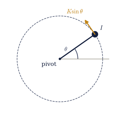
Fig. 176 The kicked rotor: a bob of moment of inertia \(I\) on a rigid massless rod, free to rotate about the pivot (no gravity), with instantaneous angle \(\theta\) measured from the horizontal axis and angular momentum \(p\). Once per period \(T\) an impulsive torque of strength \(K\sin\theta\) (amber arrow at the bob) kicks the momentum; between kicks the rotor coasts. Stroboscoping the motion at the kick period yields the standard map.#
One stepper, then three experiments, three regimes.
Part a) The map itself. Write
standard_map_ensemble(K, n_steps, theta0, p0, record_every=0), which
iterates Eq. 185 on a whole ensemble at once: apply the kick
\(p \to p + K\sin\theta\) and then the free rotation \(\theta \to \theta + p\)
modulo \(2\pi\) to every member simultaneously, and return the final
\((\theta, p)\) together with each orbit’s largest \(|p|\) along the way. Do
not wrap the momentum: unbounded \(|p|\) growth is the signature of a
broken transport barrier, which is precisely what the next two parts watch
for. When record_every is positive, also return \(\langle p^2 \rangle\)
sampled at that stride, which Part d) fits.
Write this one yourself — the implementation is the lesson.
Part b) The near-integrable limit and the resonance width. At
\(K = 0.05\), iterate an ensemble of \(100\) orbits started on the resonant
torus (\(p_0 = 0\), angles numpy.linspace(0.1, 2π-0.1, 100)) for \(5000\)
steps of Eq. 185 with your standard_map_ensemble, and record each
orbit’s maximum \(|p|\) excursion. Chirikov’s pendulum approximation says the resonance at
\(p = 0\) becomes an island of half-width exactly \(2\sqrt K\); verify the
ensemble’s largest excursion lands between \(0.8\) and \(1.05\) times
\(2\sqrt K = 0.447\): the orbits fill the island right up to its
separatrix and are stopped there by the surviving KAM curves.
Part c) The last torus. Iterate the same ensemble with your
standard_map_ensemble at \(K = 0.9\) (just below Greene’s \(K_c = 0.9716\))
and at \(K = 1.2\) (just above) for \(5000\) steps, reading off each run’s
maximum \(|p|\). Verify the confinement verdict: at \(K = 0.9\) the maximum \(|p|\)
over the whole ensemble stays below \(2\pi\) (some KAM curve, the
golden-mean torus among the last, still bars the first cylinder period),
while at \(K = 1.2\) it exceeds \(2\pi\) — the barrier is gone and transport
is global. Plot the four phase portraits \(K = 0.5, 0.9, 1.2, 2.0\) (a
\(24\times24\) grid of initial conditions, \(400\) strobe points each,
\(p\) wrapped to \([-\pi,\pi]\) for display) to watch the sea swallow the
curves.
Part d) Deterministic diffusion. Far above \(K_c\) the momentum walk
should be diffusive with \(D \approx K^2/4\). The Bessel-function
correlation corrections vanish at zeros of \(J_2\), so measure exactly
there: at \(K = 8.4172\) (the second zero, from
scipy.special.jn_zeros(2, 2)), evolve \(20\,000\) orbits from uniformly
random seeded angles (\(p_0 = 0\)) for \(2000\) steps, recording
\(\langle p^2 \rangle\) every \(100\). Verify (i) growth is diffusive: the
numpy.polyfit slope of \(\ln\langle p^2\rangle\) against \(\ln n\) is \(1\)
within \(\pm 0.05\), and (ii) the measured \(D = \langle p^2\rangle / (2n)\)
at \(n = 2000\) matches the quasilinear \(K^2/4\) to within \(15\%\): a
deterministic map, diffusing like a random walk, at the rate a
random-phase argument predicts.
With your assistant
The four-panel phase-portrait grid of Part c) is honest boilerplate: describe the layout to your assistant (a 24×24 grid of initial conditions on the cylinder, 400 strobe points each, momentum wrapped to \([-\pi,\pi]\), one panel per \(K\)) and let it write the plotting loop. The check is yours, and it is physical: rerun Part b) at \(K = 0.02\) and confirm the island’s measured half-width still tracks \(2\sqrt{K} = 0.283\). The scaling law, not the plot, is the physics.
K=0.05: max excursion / 2√K = 1.0009
K=0.9 : ensemble max |p| = 2.240 (2π = 6.283)
K=1.2 : ensemble max |p| = 11.551
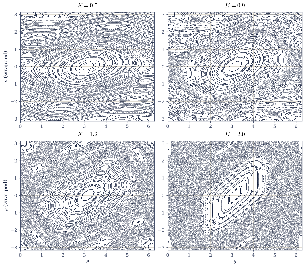
Fig. 177 Phase portraits of the standard map at \(K=0.5\), \(0.9\), \(1.2\), and \(2.0\): a \(24\times24\) grid of initial conditions on the cylinder, each iterated 400 steps, with momentum wrapped to \([-\pi,\pi]\) for display. At \(K=0.5\) the primary island at \(p=0\) sits among many surviving KAM curves; at \(K=0.9\), just below Greene’s \(K_c=0.9716\), the last horizontal curves are visibly strained but still bar vertical transport; at \(K=1.2\) they are gone and a connected chaotic sea spans the cylinder around the surviving islands; at \(K=2.0\) the sea dominates.#
log-log growth slope: 0.998 (diffusive = 1)
D measured 18.02 vs quasilinear K²/4 = 17.71 (ratio 1.017)
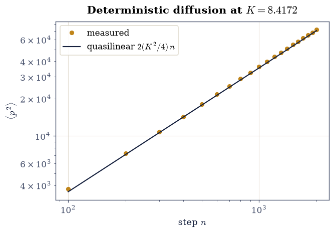
Fig. 178 Deterministic diffusion of the standard map at \(K=8.4172\) (the second zero of \(J_2\), where the leading correlation correction to the diffusion coefficient vanishes): the ensemble-averaged \(\langle p^2\rangle\) of 20,000 orbits against step number on log–log axes, beside the quasilinear prediction \(2Dn\) with \(D=K^2/4\). The measured log–log slope is \(0.996\) and the coefficient matches quasilinear theory to under two percent: a fully deterministic map executing a textbook random walk.#
✓ the K = 0.05 island fills to its separatrix: maximum excursion matches Chirikov's half-width 2√K [ratio = 1.001]
✓ the last KAM torus holds at K = 0.9 and is gone at K = 1.2, bracketing Greene's K_c = 0.9716 [max|p|: 2.24 vs 11.55, barrier 2π = 6.28]
✓ above K_c the momentum spread grows linearly in n: deterministic motion, diffusive bookkeeping [slope = 0.998]
✓ and at a J_2 zero the diffusion coefficient is quasilinear K²/4, as the random-phase argument predicts [got 18.0181 vs expected 17.7125 (rtol=0.15, atol=1e-09)]
True
Exercise 6 — Lorenz: measuring the butterfly#
The final act moves from maps to a flow. The Lorenz system Eq. 186 at \((\sigma, \rho, \beta) = (10, 28, 8/3)\) is dissipative (volumes contract at the constant rate \(\sigma + 1 + \beta = 41/3\) per time unit), so trajectories fall onto an attractor; the surprise of 1963 is that the attractor is neither a point nor a loop but a strange set on which motion separates exponentially forever. The rate of that separation is the largest Lyapunov exponent, \(\lambda_1 \approx 0.9056\) at these parameters, and measuring it means keeping the companion trajectory inside the linear regime the exponent describes: the renormalization interval \(\tau\) of the theory section has to be short enough that the separation never approaches the attractor’s own size (of order \(40\)), and the rescaled offset \(d_0\) small enough to start deep below it.
Part a) The attractor and the butterfly effect. Integrate
Eq. 186 with scipy.integrate.solve_ivp (RK45,
rtol=1e-12, atol=1e-14) from \((1, 1, 20)\): discard \(25\) time units of
transient, then follow the attractor for \(25\) more from the landing state
\(\mathbf s_0\), sampling \(2500\) points, and plot the \(x\)–\(z\) butterfly.
Repeat from \(\mathbf s_0 + (10^{-9}, 0, 0)\) and plot
\(\ln\lVert\Delta\mathbf s(t)\rVert\): the separation must grow linearly
in the log until it saturates at the attractor’s size. Fit the growth
rate over the window from \(t = 2\) until the separation first exceeds
\(1\) (numpy.polyfit, degree 1).
Part b) The measurement. Write
benettin_lambda1(s_start, tau=0.4, n_intervals=750, d0=1e-8): advance a
reference trajectory and a companion offset by \(d_0\) through one interval
\(\tau\) each, add \(\ln(d/d_0)\) to a running sum, then pull the companion
back to distance \(d_0\) along the current separation direction and repeat,
returning the mean log-growth per unit time.
Write this one yourself — the implementation is the lesson.
Part c) The exponent, twice. Measure \(\lambda_1\) with it (\(\tau = 0.4\),
\(750\) renormalization intervals: \(300\) time units on the attractor) and
verify it against the literature value
\(0.9056\) to rtol=5e-2; then verify the cross-method consistency: the
Part a) divergence-fit rate agrees with the Benettin value to
atol=0.15. Two measurements of one number, one from a single
separation event, one from three hundred renormalized ones.
Part d) Lorenz’s own argument. Record every successive local maximum
of \(z(t)\) over \(120\) time units and plot each maximum against the next:
the three-dimensional flow collapses onto a one-dimensional tent-shaped
return map (this is Lorenz’s 1963 construction). Estimate the local slope
magnitudes with numpy.diff on the sorted pairs and verify that at least
\(98\%\) exceed \(1\): an everywhere-expanding return map can hold no stable
periodic orbit, which is the cleanest one-line proof that the attractor’s
irregularity is structural, not transient.
Text(0.5, 1.0, 'The Lorenz attractor')
Fig. 179 The Lorenz attractor at \((\sigma,\rho,\beta)=(10,28,8/3)\), projected on the \(x\)–\(z\) plane: 25 time units of post-transient trajectory from \((1,1,20)\), integrated by RK45 at rtol \(10^{-12}\). The two lobes are circulations of opposite sense; the trajectory switches lobes irregularly and never closes.#
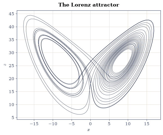
Fig. 180 The Lorenz attractor at \((\sigma,\rho,\beta)=(10,28,8/3)\), projected on the \(x\)–\(z\) plane: 25 time units of post-transient trajectory from \((1,1,20)\), integrated by RK45 at rtol \(10^{-12}\). The two lobes are circulations of opposite sense; the trajectory switches lobes irregularly and never closes.#