0.2 Root-Finding

Elementary Computational Physics

Volume 0 — Mathematical & Computational Foundations Notebook 0.2

Solving f(x)=0 when there is no formula: bisection, Newton, and the secant method — their convergence orders, their failure modes, and the engine behind the transcendental equations of quantum mechanics.

Level · intermediate   •   Est. · 80–110 min

Raymond Amador v1.4.0  ·  2026-07-31  ·  CC BY 4.0 (text) / MIT (code)

Notebook overview

We learned what a root is in secondary school: a value \(x_\star\) with \(f(x_\star)=0\), and how to find one when the algebra cooperates: factor the quadratic, invert the function. The question then becomes what to do when it doesn’t: when \(f\) has no closed-form inverse, which is the overwhelmingly common case in physics. How does one actually find \(x_\star\) then, how fast, and how can it go wrong?

This notebook builds the three classical answers from scratch (bisection, Newton’s method, and the secant method) and measures the property that separates them: their order of convergence, how quickly the error shrinks per step. We will see bisection crawl (one bit at a time, but never failing), Newton sprint (doubling its correct digits each step) and then spectacularly fail by cycling forever, and the secant method land in between at a rate set by the golden ratio. We close on scipy.optimize.brentq, the safe-and-fast hybrid that is the course’s default.

This is foundational in the literal sense: the solver we build here is the engine for the transcendental eigenvalue equations of quantum mechanics: the finite square well in §6.11, and \(\tan x = x\) for the infinite spherical well in §6.16 (which we solve, as a preview, in Exercise 7), and for the orbital turning points of §2.4. Familiar goal, unfamiliar machinery.

How to read the checks. Each exercise ends with a validate call that compares our result to an independent truth: a known root, a predicted convergence order, an exact special value. A ✓ is strong evidence we got it right; a ✗ is not a verdict but a prompt to locate the discrepancy (a bracket that strayed across an asymptote, an order estimated on the noisy tail near machine precision, a derivative typo). Passing is strong evidence, not proof.

Scope. A working review, not a numerical-analysis course. For the full treatment see Press et al., Numerical Recipes, ch. 9 [PTVF07], and Higham [Hig02] on the floating-point limits that set the accuracy floor (§0.1).

Theory in brief

The problem and two families of method

Given continuous \(f\), find \(x_\star\) with \(f(x_\star)=0\). The methods split into two families. Bracketing methods keep an interval known to contain a root and shrink it: guaranteed to converge, but slowly. Open (iterative) methods generate a sequence \(x_n \to x_\star\) from a formula: fast, but with no safety net: they can diverge, cycle, or land on the wrong root.

Bisection

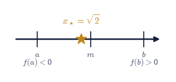
If \(f(a)\,f(b) < 0\) then \(f\) has a root in \([a,b]\) (intermediate value theorem). Bisection evaluates the midpoint \(m=\tfrac12(a+b)\) and keeps whichever half still brackets the sign change. After \(n\) steps the bracket width is

(8)\[(b-a)_n = \frac{(b-a)_0}{2^{\,n}},\]

so the width halves every step: linear convergence, exactly one bit of accuracy per evaluation, but guaranteed. (A subtlety we exploit below: the bracket width halves cleanly, while the midpoint error can jump around inside the shrinking bracket, so convergence is best measured by the width.)

Newton’s method

Newton linearises \(f\) at the current guess and steps to where the tangent crosses zero:

(9)\[x_{n+1} = x_n - \frac{f(x_n)}{f'(x_n)}.\]

Near a simple root it converges quadratically: the error squares each step (\(e_{n+1}\sim e_n^2\)), so the number of correct digits roughly doubles per iteration (a Taylor expansion of \(f\) about the root shows it; Press et al., Numerical Recipes, §9.4, carry the expansion out in full). The price: it needs \(f'\), it needs a good starting guess, and it fails outright where \(f'=0\) or when the geometry sends it cycling or diverging.

The secant method

When the derivative is unavailable or expensive, we can approximate it from the two previous iterates. Replacing \(f'(x_n)\) in Eq. 9 by a finite difference gives the secant method:

(10)\[x_{n+1} = x_n - f(x_n)\,\frac{x_n - x_{n-1}}{f(x_n) - f(x_{n-1})}.\]

Because it needs no derivative, it is often the practical choice; the price for that convenience is a slightly slower convergence order, the golden ratio \(\varphi = \tfrac{1+\sqrt5}{2}\approx 1.618\): still superlinear, sitting neatly between bisection’s linear crawl and Newton’s quadratic sprint. (The order follows from the two-term error recursion \(e_{n+1}\sim e_n e_{n-1}\); Press et al., Numerical Recipes, §9.2, sketch the argument.)

Measuring the order of convergence

The order \(p\) is defined by \(e_{n+1} \approx C\,e_n^{\,p}\) with \(e_n = |x_n - x_\star|\). Taking logs of three consecutive errors eliminates the constant \(C\) and gives an estimator

(11)\[p \approx \frac{\ln(e_{n+1}/e_n)}{\ln(e_n/e_{n-1})}.\]

We must read \(p\) from the mid-range iterates: the first few have not settled into the asymptotic regime, and the last few sit on the machine-precision floor (§0.1), where \(e_n\) is round-off noise and the ratio is meaningless.

Failure modes and the practical default

Newton’s failures are vivid: a step through a near-zero \(f'\) flings the iterate far away; some functions and starts make it cycle forever; others diverge. Bracketing methods are immune to these but cannot find a root without a sign change (so they miss even-multiplicity roots). The practical default is scipy.optimize.brentq, Brent’s method, which combines bisection’s guarantee with the speed of the secant / inverse-quadratic interpolation, and is what we use throughout the course.

Setup

Data and instruments only: the golden ratio \(\varphi\), which is the number the secant method’s measured order has to reproduce, and a step counter that reports where an error sequence first crosses a tolerance. The methods this notebook is about are deliberately absent: you write bisection in Exercise 1, newton and the convergence-order estimator of Eq. 11 in Exercise 3, and secant in Exercise 4.

The Setup below holds this notebook’s data and instruments — nothing you are asked to build. It is collapsed so the building stays yours; expand it whenever you want the details.

Show code cell source

Hide code cell source

import numpy as np
import matplotlib.pyplot as plt
from scipy.optimize import brentq

from ecp import draw, validate
from ecp.animate import show

PHI = (1 + np.sqrt(5)) / 2  # data: golden ratio, the secant method's order


# instrument: a step counter for the cost comparison of Exercise 4 — reading
# off where an error sequence first crosses a tolerance is array bookkeeping,
# not the root-finding craft this notebook teaches.
def iterations_to_tol(errors, tol=1e-12):
    """Number of steps until the error first drops below a tolerance.

    Parameters
    ----------
    errors : array_like
        The per-step error sequence.
    tol : float, optional
        Target tolerance (default 1e-12).

    Returns
    -------
    int
        The step count to reach ``tol``.
    """
    below = np.where(np.asarray(errors) < tol)[0]
    return int(below[0]) if below.size else len(errors)

Exercise 1 — Bisection from scratch

Recall the bracketing guarantee behind Eq. 8: if \(f(a)f(b)<0\), a root lies between, and halving the bracket can never lose it. The test function here is \(f(x)=x^2-2\), whose positive root is the irrational \(\sqrt{2}\): a number with no finite decimal, reached below purely by repeated sign tests, and known in advance, which is what makes it a fair test. Fig. 14 shows the geometry of a single step.

1. Write bisection(f, a, b, tol=1e-13, maxit=200): evaluate the midpoint \(m=\tfrac12(a+b)\), keep whichever half still carries the sign change, and stop when the bracket is narrower than tol; return the final midpoint together with the midpoint and bracket-width histories (the two records Exercises 2 and 3 measure). Refuse a bracket with \(f(a)f(b)\ge0\) — without a sign change Eq. 8 guarantees nothing. Write this one yourself — the implementation is the lesson.

2. Run it on \([a,b]=[1,2]\) (note \(f(1)=-1<0\), \(f(2)=2>0\)) to a tight tolerance.

3. Confirm the result equals \(\sqrt{2}\).

Fig. 14 Bisection geometry on \(f(x)=x^2-2\): the bracket \([a,b]\) straddles the root \(x_\star=\sqrt{2}\) because \(f(a)<0\) and \(f(b)>0\) (opposite signs), and the midpoint \(m=\tfrac12(a+b)\) replaces whichever endpoint keeps the sign change, halving the bracket each step per Eq. 8.

Solution

bisection root = 1.4142135623730780
√2             = 1.4142135623730951
iterations     = 45

Validation 1

✓  bisection converges to √2   [got 1.41421 vs expected 1.41421 (rtol=1e-10, atol=1e-09)]

True

Exercise 2 — Bisection converges linearly (measured correctly)

The theory, Eq. 8, says the bracket width is \((b-a)_0/2^n\). This exercise checks that directly, and makes a methodological point. The right quantity to track for bisection is the bracket width, which halves cleanly every step; the midpoint error is noisy, because the midpoint can land very close to the root on one step and then jump away on the next, so error ratios give a meaningless “order”. This is itself worth seeing.

1. From the bracket history of Exercise 1, form the width ratios \((b-a)_{n+1}/(b-a)_n\) (an array shift-and-divide) and confirm they equal \(\tfrac12\).

2. Plot the bracket width against iteration on a log \(y\)-axis (matplotlib.pyplot.semilogy): a straight line of slope \(-\log 2\), the signature of linear convergence (Fig. 15).

width ratios (first 6): [0.5 0.5 0.5 0.5 0.5 0.5]
mean width ratio       = 0.500000000000

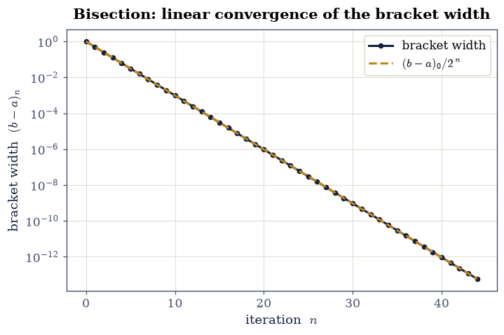
Fig. 15 Bisection bracket width versus iteration \(n\) for \(f(x)=x^2-2\), on a logarithmic \(y\)-axis: the width follows \((b-a)_0/2^{\,n}\) (dashed) as a straight line of slope \(-\log 2\), the hallmark of linear convergence — one bit of accuracy per function evaluation.

Validation 2

✓  the bracket width halves each step   [max|Δ| = 0 (rtol=1e-06, atol=1e-09)]

True

Exercise 3 — Newton’s method and quadratic convergence (worked)

Newton’s update, Eq. 9, steps along the tangent. Near a simple root it converges quadratically, Eq. 11 with \(p=2\): the error squares, so correct digits double per step, and that predicted \(p=2\) is the number the measurement below has to return. The same test function serves, \(f(x)=x^2-2\), whose derivative \(f'(x)=2x\) is available in closed form (Newton needs one) and whose root \(\sqrt2\) is again known in advance, so the error \(e_n=|x_n-\sqrt2|\) is exactly computable at every step.

1. Write newton(f, fprime, x0, tol=1e-14, maxit=100): iterate Eq. 9 until \(|f(x)|\) or the step size falls below tol, returning the root and the full iterate history. Write this one yourself — the implementation is the lesson.

2. Iterate from \(x_0=2\) and record the iterates.

3. Write convergence_order(hist, root, lo=1e-13, hi=0.5), the three-error estimator Eq. 11 applied to every consecutive triple of errors whose members all lie inside the window [lo, hi]: that window is what excludes the head (not yet in the asymptotic regime) and the tail (round-off noise on the machine-precision floor of §0.1).

4. Estimate Newton’s order with it, taking the median over the surviving triples.

5. Plot Newton’s error against iteration alongside bisection’s on the same log axes (Fig. 16): the plunge versus the straight-line crawl.

Newton root  = 1.4142135623730951   in 5 steps
measured convergence order p = 1.992   (theory: 2)

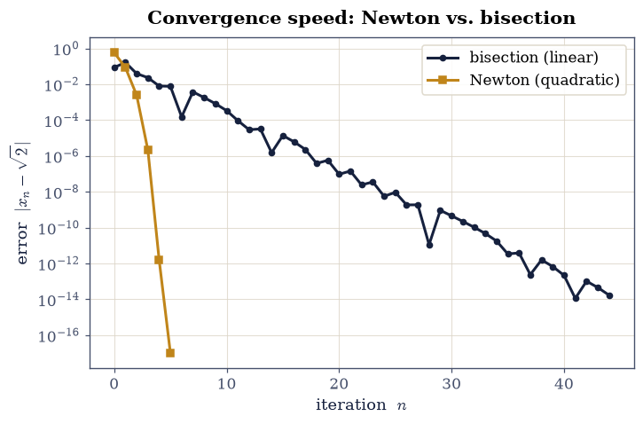
Fig. 16 Error \(|x_n-\sqrt{2}|\) versus iteration for the same root of \(f(x)=x^2-2\), log \(y\)-axis: Newton (amber) converges quadratically — the error plunges, correct digits doubling each step — while bisection (dark) descends as a straight line, one bit per step, until both reach the machine-precision floor of §0.1.

Validation 3

✓  Newton converges quadratically (order ≈ 2)   [got 1.99184 vs expected 2 (rtol=1e-06, atol=0.3)]

True

Exercise 4 — The secant method and the golden ratio

The secant update, Eq. 10, is Newton with the derivative replaced by a finite difference over the last two iterates: no \(f'\) required. Its order is the golden ratio \(\varphi=\tfrac{1+\sqrt5}{2}\approx1.618\) (the Setup’s PHI), between bisection’s \(1\) and Newton’s \(2\) — the prediction the measurement has to reproduce. Because two iterates are needed before the first update, the method is seeded with a pair of guesses rather than one.

1. Write secant(f, x0, x1, tol=1e-14, maxit=100): iterate Eq. 10, carrying the last two points and their function values forward, and return the root and the iterate history. Write this one yourself — the implementation is the lesson.

2. Iterate on \(f(x)=x^2-2\) from \(x_0=2,\ x_1=1.5\), and estimate the order with the convergence_order you wrote in Exercise 3 (read over the mid-range iterates: the tail is noisy near machine precision).

3. Count iterations to reach a \(10^{-12}\) error for all three methods — the bisection of Exercise 1, the newton of Exercise 3, and the secant just built — and compare them in a bar chart (Fig. 17): bisection’s many steps against the handful Newton and the secant need.

secant root = 1.4142135623730954   in 5 steps
measured convergence order p = 1.667   (theory: φ = 1.618)
iterations to 1e-12 — bisection 37, Newton 5, secant 6

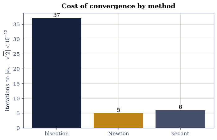
Fig. 17 Function evaluations to reach a \(10^{-12}\) error in \(\sqrt{2}\) for the three hand-coded methods: bisection’s guaranteed-but-slow linear convergence costs many steps, while Newton (quadratic) and the secant method (order \(\varphi\)) reach the same accuracy in a handful — the price of bisection’s safety is speed.

Validation 4

✓  the secant method's order is the golden ratio φ   [got 1.66662 vs expected 1.61803 (rtol=1e-06, atol=0.3)]

True

Exercise 5 — When Newton fails (the cautionary tale)

Newton’s speed comes with no guarantee. With the wrong function or start, the update Eq. 9 can cycle forever or diverge. The classic cycle: on \(f(x)=x^3-2x+2\) from \(x_0=0\), Newton maps \(0\to1\to0\to1\to\cdots\) and never converges, even though the function has a real root near \(-1.77\).

1. Iterate Newton on \(f(x)=x^3-2x+2\) from \(x_0=0\) and confirm the sequence is \(0,1,0,1,\dots\).

2. Show the near-zero-derivative overshoot too: start near the critical point \(f'(x)=0\) at \(x=\sqrt{2/3}\approx0.8165\) and watch a single step fling the iterate far across the axis. Fig. 18 draws the tangent steps of the cycle.

Newton iterates from x0=0:  [0. 1. 0. 1. 0. 1. 0. 1.]
Newton iterates from x0=0.82 (near f'=0):  [  0.82  -52.167 -34.786 -23.204 -15.49  -10.358  -6.955]

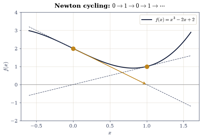
Fig. 18 Newton’s method cycling on \(f(x)=x^3-2x+2\) from \(x_0=0\): the tangent at \(x=0\) (per Eq. 9) meets the axis at \(x=1\), the tangent at \(x=1\) returns to \(x=0\), and the iterate bounces between the two (amber points) forever — a stable 2-cycle that never reaches the genuine root near \(x\approx-1.77\).

Validation 5

✓  Newton cycles 0,1,0,1,… and never converges from this start   [first iterates = [0. 1. 0. 1. 0. 1.]]
✓  from a start near f'=0 the near-zero slope flings the iterate far from the root   [last iterate = -6.955]

True

Exercise 6 — Newton’s basins of attraction (worked animation)

Newton’s update Eq. 9 is arithmetic, so it runs unchanged on the complex function \(f(z)=z^3-1\), whose three roots are the cube roots of unity. Every starting point in the plane converges to one of the three — but the map “start \(\to\) which root” has a fractal boundary: near the borders, points arbitrarily close together end up at different roots. This is the famous Newton fractal: a familiar method producing astonishing structure.

1. Iterate Newton’s update for \(f(z)=z^3-1\) on a grid of complex starting points (numpy.meshgrid over the plane).

2. Colour each start by the root it reaches (numpy.argmin of the distances to the three roots) and animate the basin map sharpening as the iteration count grows (Fig. 19).

3. Validate the mathematics of the data: starts placed next to each root converge to that root, and every limit Newton finds is a genuine root of \(f\).

Once Loop Reflect

Fig. 19 Animation of Newton’s basins of attraction for \(f(z)=z^3-1\) in the complex plane: each pixel is a starting point, coloured by which cube root of unity \(\{1,\,e^{2\pi i/3},\,e^{4\pi i/3}\}\) Newton’s iteration Eq. 9 reaches, with the colouring sharpening as the iteration count grows — the basin boundaries are a fractal, where starts arbitrarily close together fall to different roots.

Validation 6

✓  starts next to each root converge to that root   [max|Δ| = 4.96507e-16 (rtol=1e-06, atol=1e-09)]
✓  every basin converges to a genuine root of f(z)=z³−1   [max|Δ| = 2.48253e-16 (rtol=1e-06, atol=1e-08)]

True

Exercise 7 — The transcendental root that QM needs

Here is that forward promise, made concrete. In §6.16 the energy levels of the infinite spherical well (angular momentum \(\ell=1\)) are the roots of the transcendental equation \(\tan x = x\): no formula gives them; one must root-find. This exercise finds the first nonzero root, \(x_\star \approx 4.4934\).

1. Plot \(y=\tan x\) and \(y=x\) and locate the first few intersections graphically (Fig. 20), noting the asymptotes of \(\tan\) at \(x=(k+\tfrac12)\pi\): a bracket must not straddle one.

2. The first nonzero root lies between the asymptotes at \(\pi/2\) and \(3\pi/2\); bracket it safely inside \((\pi,\,3\pi/2)\) (e.g. \([4.0,\,4.6]\), clear of the asymptote at \(3\pi/2\approx4.712\)), and solve with the bisection you wrote in Exercise 1.

3. Draw the bracket closing on the root: a static “ladder” of the successive intervals \([a,b]_n\), each row half the width of the one above (Fig. 21). (No animation here: the lesson is the nesting of intervals, which a still ladder shows at a glance.)

The validation checks the root, so a ✗ means “check the bracket (did it cross the \(\tan\) asymptote?) or the iteration.”

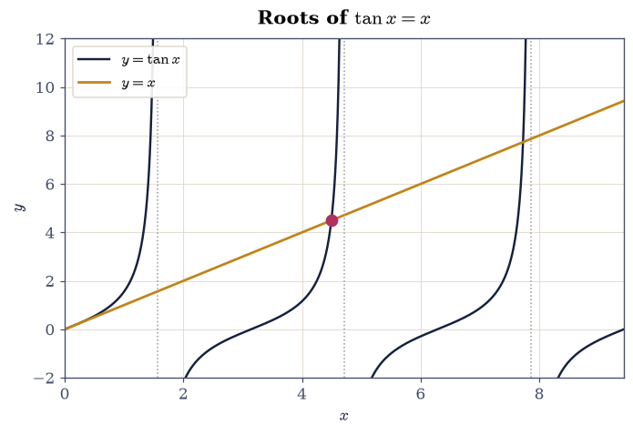
Fig. 20 Graphical construction of the roots of \(\tan x = x\): the line \(y=x\) (amber) crosses each branch of \(y=\tan x\) (dark) once, with the vertical asymptotes of \(\tan\) at \(x=(k+\tfrac12)\pi\) (dotted) separating the branches; the first nonzero intersection, \(x_\star\approx4.4934\) (marked), is the \(\ell=1\) level of the infinite spherical well of §6.16.

first nonzero root of tan x = x:  4.4934094579
reference value:                  4.4934094579

Part 3 reconstructs the bracket history \([a,b]_n\) from the bisection run and draws it as a static ladder: successive rows, each interval half the last, converging on the root.

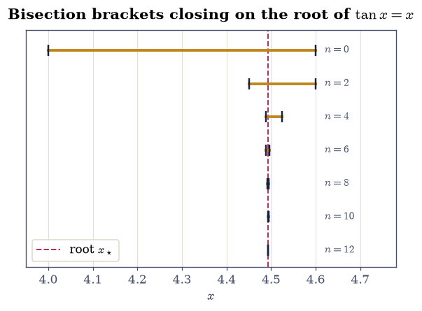
Fig. 21 Successive bisection brackets \([a,b]_n\) (amber bars, endpoints ticked) closing on the first nonzero root of \(\tan x = x\) (dashed line, \(x_\star\approx4.4934\)): rows descend with iteration \(n\) and each interval is half the width of the one above per Eq. 8, so the bracket nests geometrically onto the root while staying inside \((\pi,3\pi/2)\), clear of the asymptote.

Validation 7

✓  first nonzero root of tan x = x   [got 4.49341 vs expected 4.49341 (rtol=1e-08, atol=1e-09)]

True

Exercise 8 — Brent’s method: safety and speed (synthesis)

In practice one neither hand-codes bisection nor risks Newton’s failures: one calls Brent’s method, scipy.optimize.brentq. It keeps a bracket (so it inherits bisection’s guarantee, Eq. 8) but interpolates with secant / inverse-quadratic steps (so it inherits their speed). It is the course default (for orbital turning points in §2.4 and the eigenvalue equations of §6), and it needs only a sign-changing bracket.

1. Re-solve the roots of Exercises 1 and 7 with scipy.optimize.brentq.

2. Confirm it lands on the same values the hand-coded solvers found.

brentq √2          = 1.4142135623731364
brentq tan x = x   = 4.4934094579

Validation 8

✓  Brent's method matches √2   [got 1.41421 vs expected 1.41421 (rtol=1e-10, atol=1e-09)]
✓  Brent's method matches the hand-coded tan x = x root   [got 4.49341 vs expected 4.49341 (rtol=1e-10, atol=1e-09)]

True

Notebook summary

• Bisection (linear convergence) and Newton’s method (quadratic, measured order \(\approx2\)) converging to \(\sqrt2\); the secant method at the golden-ratio order \(\approx1.618\).

• Where Newton fails and its fractal basins of attraction; a transcendental root needed in quantum mechanics; and Brent’s method as the safe, fast default (scipy.optimize.brentq).

Outlook

• Multiple roots. At a repeated root \(f'\) also vanishes and Newton’s convergence degrades from quadratic to linear; the modified update \(x_{n+1}=x_n - m\,f/f'\) (with multiplicity \(m\)) restores it.

• Systems of equations. The multivariate Newton replaces \(f'\) with the Jacobian matrix and solves a linear system each step: the engine behind shooting methods and behind locating the equilibria of §2.7.

• Continuation / homotopy. Track a root as a parameter varies, using each solution as the start for the next: invaluable when a good initial guess is otherwise hard to find.

• Forward links. §2.4 (turning points via brentq on \(E - V_{\rm eff}\)); §6.11, §6.16 (transcendental eigenvalues); §6.17 (shooting for the hydrogen radial equation).

References

[Hig02]

Nicholas J. Higham. Accuracy and Stability of Numerical Algorithms. Society for Industrial and Applied Mathematics (SIAM), 2 edition, 2002.

[PTVF07]

William H. Press, Saul A. Teukolsky, William T. Vetterling, and Brian P. Flannery. Numerical Recipes: The Art of Scientific Computing. Cambridge University Press, 3 edition, 2007.

Take this notebook with you

Use the download button (↓) in the toolbar above to save this notebook and run it yourself. The published notebooks ship without worked solutions; if you would like the reference solutions — to teach from or to check your own work — get in touch: hello@ramador.me.