3.12 The Relativistic Formulation of Maxwell’s Equations

3.12 The Relativistic Formulation of Maxwell’s Equations#

    Elementary Computational Physics
  

Volume III — Classical Electrodynamics Notebook 3.12

The summit: spacetime, the field tensor, and Maxwell's four equations in two lines. Electricity and magnetism turn out to be a single object seen from different frames — magnetism is what an electric field looks like to a moving observer.

Level · advanced • Est. · 180–220 min

    Raymond Amador
    v1.4.0  ·  2026-07-31  · 
          CC BY 4.0 (text) / MIT (code)
  

Notebook overview#

This is the longest and most demanding notebook of the volume, and the most rewarding. It asks two unfamiliar things at once, to think in four dimensions and to think in tensors, and in return the eleven notebooks before it snap into a single structure. The claim is audacious and exact: electricity and magnetism are not two phenomena but one, a single geometric object, and which part of it you call “electric” and which “magnetic” depends only on how you are moving. Magnetism is what an electric field looks like to a moving observer.

A note on reading order: this notebook sits in Volume III as the capstone of electrodynamics, but it leans on special relativity. If you are meeting relativity for the first time, you may prefer to read the special-relativity notebooks of Volume IV (§4.1–§4.5) first and return here afterwards. We develop just enough relativity inline for the notebook to stand on its own, but the fuller story is in Volume IV. In particular the four-vector and np.einsum machinery we use inline here (the metric \(\eta\), the contraction \(\eta_{\mu\nu}a^\mu b^\nu\), raising and lowering) is developed carefully, from the geometry up, in §4.3; a reader who wants the index-string grammar spelled out should look there.

The road there starts from the crisis §3.8 left open. Maxwell’s equations pick out a speed \(c=1/\sqrt{\mu_0\varepsilon_0}\), but a speed relative to what? Einstein’s answer, that \(c\) is the same in every inertial frame and space and time themselves transform to make it so, forces the Lorentz transformation, four-vectors, and a four-dimensional spacetime. We develop only as much special relativity as we need to rewrite electrodynamics; the full development is Volume IV, which we cross-reference. With that groundwork we build the field tensor \(F^{\mu\nu}\), the six numbers of \(\mathbf E\) and \(\mathbf B\) assembled into one antisymmetric object, collapse all four Maxwell equations into two tensor lines, and watch a boost mix \(\mathbf E\) and \(\mathbf B\) into each other. We end with the two Lorentz invariants every observer agrees on; with the gauge arc’s final turn: the freedom of §3.6 and the tool of §3.8 are revealed as structure, \(F^{\mu\nu}=\partial^\mu A^\nu-\partial^\nu A^\mu\) being manifestly gauge-invariant, with a forward pointer to where gauge invariance becomes physics (Vol V) and back to its Noether root (§2.2); and with the field’s own stress–energy tensor \(T^{\mu\nu}\) — energy density, Poynting flux, and Maxwell stress as one object — put to work until a surface integral of field stress alone reproduces Coulomb’s force between two charges.

We work in SI units with the metric signature \((-,+,+,+)\), used throughout. (At this altitude Gaussian units are tidier, hiding the factors of \(c\); we keep SI for continuity and note where \(c\) would vanish.) The one animation is genuinely warranted: a boost continuously sweeping a pure electric field into a mixture of electric and magnetic, the unification set in motion. Everything else is a still.

How to read the checks. Each exercise ends with a validate call against an independent fact: the spacetime interval invariant under a boost, the four-velocity norm \(-c^2\), the field tensor antisymmetric, the covariant equations reproducing the four 3-vector ones, the field invariants frame-independent, \(F^{\mu\nu}\) unchanged by a gauge transformation. A ✓ is strong evidence; a ✗ is a prompt to locate the discrepancy, not a verdict.

Scope. Enough relativity to recast electrodynamics, not a relativity course (that is Vol IV). See Nolting, Theoretical Physics 3/4 [Nol16]; Griffiths, Introduction to Electrodynamics [Gri17] (ch. 12); Jackson [Jac98] (ch. 11); Landau & Lifshitz, The Classical Theory of Fields [LL80].

Theory in brief#

The crisis that forces relativity#

Maxwell’s equations give one speed \(c=1/\sqrt{\mu_0\varepsilon_0}\) (§3.8), but Galilean velocity addition makes every speed frame-dependent. In which frame, then, is light’s speed \(c\)? The nineteenth-century answer, a luminiferous aether, failed (Michelson– Morley). Einstein’s resolution is the postulate

(255)#\[c \text{ is the same in every inertial frame,}\]

from which space and time must themselves transform.

Spacetime and the Lorentz transformation#

Events live in four-dimensional spacetime, \(x^\mu=(ct,x,y,z)\), with the invariant interval set by the Minkowski metric \(\eta=\mathrm{diag}(-1,1,1,1)\),

(256)#\[s^2 = \eta_{\mu\nu}x^\mu x^\nu = -c^2t^2+x^2+y^2+z^2 .\]

A boost along \(x\) at speed \(v\) (\(\beta=v/c\), \(\gamma=1/\sqrt{1-\beta^2}\)) is the linear map \(\Lambda\) that mixes \(t\) and \(x\) while leaving \(s^2\) unchanged.

Four-vectors#

Quantities that transform like \(x^\mu\) are four-vectors: the four-velocity \(u^\mu=\gamma(c,\mathbf v)\) with the invariant norm \(u^\mu u_\mu=-c^2\), and the two that carry electrodynamics,

(257)#\[J^\mu=(c\rho,\mathbf J), \qquad A^\mu=(V/c,\mathbf A).\]

Charge conservation and the Lorenz gauge each become a single four-divergence, \(\partial_\mu J^\mu=0\) and \(\partial_\mu A^\mu=0\).

The field tensor#

The six numbers in \(\mathbf E\) and \(\mathbf B\) are not two 3-vectors but the six independent components of one antisymmetric rank-2 tensor,

(258)#\[F^{\mu\nu}=\partial^\mu A^\nu-\partial^\nu A^\mu, \qquad F^{0i}=E_i/c, \quad F^{ij}=-\varepsilon^{ijk}B_k .\]

Written as a \(4\times4\) matrix it holds \(\mathbf E\) in its time row/column and \(\mathbf B\) in its spatial block: \(\mathbf E\) and \(\mathbf B\) are one object. Griffiths, Introduction to Electrodynamics, ch. 12, works the identification of the components out entry by entry.

Maxwell in two lines#

All four equations collapse to the sourced pair and the source-free (Bianchi) pair,

(259)#\[\partial_\mu F^{\mu\nu}=\mu_0 J^\nu, \qquad \partial^\alpha F^{\beta\gamma}+\partial^\beta F^{\gamma\alpha}+\partial^\gamma F^{\alpha\beta}=0 .\]

The first reproduces Gauss (\(\nu=0\)) and Ampère–Maxwell (\(\nu=i\)); the second reproduces \(\nabla\cdot\mathbf B=0\) and Faraday.

E and B mix under boosts#

Transforming the tensor to a boosted frame, \(F'^{\mu\nu}=\Lambda^\mu{}_\alpha \Lambda^\nu{}_\beta F^{\alpha\beta}\), mixes the fields,

(260)#\[E'_\parallel=E_\parallel,\quad \mathbf E'_\perp=\gamma(\mathbf E+\mathbf v\times\mathbf B)_\perp,\quad \mathbf B'_\perp=\gamma\Big(\mathbf B-\tfrac{1}{c^2}\mathbf v\times\mathbf E\Big)_\perp .\]

A pure Coulomb field, seen from a moving frame, acquires a magnetic component: magnetism is electricity in motion.

Gauge invariance as structure, and the invariants#

Because \(\partial^\mu\partial^\nu\chi\) is symmetric, \(F^{\mu\nu}=\partial^\mu A^\nu- \partial^\nu A^\mu\) is manifestly unchanged under

(261)#\[A^\mu \to A^\mu+\partial^\mu\chi ,\]

so the gauge freedom of §3.6 and the gauge tool of §3.8 are now seen as a structural feature of the four-potential, with the Lorenz condition \(\partial_\mu A^\mu=0\) manifestly Lorentz-invariant. From \(F^{\mu\nu}\) one builds two Lorentz scalars,

(262)#\[\mathbf E\cdot\mathbf B \;\propto\; F_{\mu\nu}\widetilde F^{\mu\nu}, \qquad E^2-c^2B^2 \;\propto\; F_{\mu\nu}F^{\mu\nu},\]

the same in every frame even as \(\mathbf E\) and \(\mathbf B\) separately change. Landau & Lifshitz, The Classical Theory of Fields, construct the dual tensor \(\widetilde F^{\mu\nu}\) and derive both invariants.

Setup#

Data and instruments only: the CODATA constants that fix \(c=1/\sqrt{\mu_0\varepsilon_0}\), the series palette, the Minkowski metric \(\eta=\mathrm{diag}(-1,1,1,1)\) that fixes this notebook’s signature, and the metric contraction \(\eta_{\mu\nu}a^\mu b^\nu\) written once as a call so the exercises read as physics rather than as index strings. This notebook’s own machinery is not here: you write the Lorentz boost \(\Lambda(\beta)\) in Exercise 1, the four-velocity \(u^\mu\) in Exercise 2, and the field tensor \(F^{\mu\nu}\) together with its inverse read-out in Exercise 3. Every boost, every mixing of \(\mathbf E\) and \(\mathbf B\), and every invariant downstream runs on those three. No randomness appears anywhere in this notebook.

The Setup below holds this notebook’s data and instruments — nothing you are asked to build. It is collapsed so the building stays yours; expand it whenever you want the details.

Movement I — Spacetime and four-vectors#

Exercise 1 — The Lorentz transformation and the invariant interval (worked)#

Special relativity begins by taking \(c\) as absolute Eq. 255 and letting space and time bend to keep it so. The carrier of that bending is the Lorentz boost \(\Lambda\), which mixes \(t\) and \(x\) but preserves the interval \(s^2=\eta_{\mu\nu}x^\mu x^\nu\) Eq. 256 (Fig. 285). What looks like a fixed time and a fixed position to one observer is a blend of both to another, yet both agree on \(s^2\). The boost here runs at \(v=0.6c\), and the three events it acts on include one sitting on the light line \(ct=x\): whatever the boost does, that event must stay on the light line, because \(c\) is the same in both frames.

Write lorentz_boost(beta), returning the \(4\times4\) matrix \(\Lambda\) of a boost along \(x\) at \(\beta=v/c\): \(\gamma=1/\sqrt{1-\beta^2}\) in the \((0,0)\) and \((1,1)\) slots, \(-\gamma\beta\) in the \((0,1)\) and \((1,0)\) slots, and the identity on \(y\) and \(z\), which a boost along \(x\) leaves alone. Write this one yourself — the implementation is the lesson, and every change of frame in this notebook goes through it.
Apply it to a set of events by matrix multiplication, events @ Λ.T, and form the interval as the contraction x @ η @ x (the Setup’s minkowski_dot) before and after, confirming \(s^2\) is unchanged while \(t\) and \(x\) individually transform.
Check that the light-line event maps to another light-line event: the speed of light is \(c\) in both frames, the whole point.

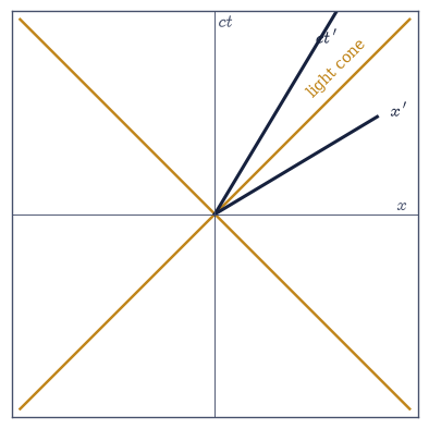
../../_images/86721345433d13c9751ea58cc9c1e48c4e601ef02def2a95db0ce5a860645bd3.png — Fig. 285 A spacetime diagram in the \((x,ct)\) plane. The light cone \(ct=\pm x\) (amber) separates past and future; a boost at \(v=0.6c\) tilts the time axis \(ct'\) and space axis \(x'\) symmetrically toward the cone (dark), the hallmark of the Lorentz transformation. The light cone is left invariant: light travels at \(c\) for every observer, which is what forces the tilt.#

interval s² before: [-0.75 -2.15  0.  ]
interval s² after : [-0.75 -2.15  0.  ]
light ray ct=x before (1.000, 1.000); after (0.500, 0.500) → still ct'=x' (c invariant: True)

Validation 1#

✓  the spacetime interval is Lorentz-invariant   [max|Δ| = 0 (rtol=1e-10, atol=1e-09)]
✓  a light ray maps to a light ray — c is the same in both frames   [got 0.5 vs expected 0.5 (rtol=1e-10, atol=1e-09)]

True

Exercise 2 — Four-vectors: velocity, current, potential (worked)#

Anything that transforms under \(\Lambda\) like the position \(x^\mu\) is a four-vector, and the Minkowski norm \(a^\mu a_\mu\) is then a scalar every observer agrees on. The four-velocity \(u^\mu=\gamma(c,\mathbf v)\) Eq. 257 has the fixed norm \(u^\mu u_\mu=-c^2\), a compact way of saying everything advances through spacetime at speed \(c\). The same packaging gives the four-current \(J^\mu=(c\rho,\mathbf J)\) and four-potential \(A^\mu=(V/c,\mathbf A)\), and in this language two scattered facts of §3.8, charge conservation and the Lorenz gauge, each become a single four-divergence.

The four-potential used below is a transverse plane wave, \(A^\mu=a^\mu\cos(kx-\omega t)\) with \(a^\mu=(0,0,a_y,0)\) and \(\omega=ck\): because \(a^\mu\) has no time or \(x\) component, \(\partial_\mu A^\mu=(1/c)\partial_t A^0+\partial_x A^1\) vanishes identically, so the Lorenz condition is satisfied and the numerics should see it.

Write four_velocity(v), returning \(u^\mu=\gamma(c,\mathbf v)\) Eq. 257 for an ordinary 3-velocity \(\mathbf v\), with \(\gamma=1/\sqrt{1-\mathbf v\cdot\mathbf v/c^2}\).
For \(v=0.6c\) along \(x\), verify \(u^\mu u_\mu=-c^2\) by contracting it with the metric, np.einsum("m,mn,n->", u, η, u) (the Setup’s minkowski_dot).
Form the four-divergence \(\partial_\mu A^\mu\) of that plane-wave four-potential by differencing each component with numpy.gradient along its own axis and summing, confirming the Lorenz condition holds — the single equation \(\partial_\mu A^\mu=0\) standing in for \(\nabla\cdot\mathbf A+\tfrac1{c^2}\partial_t V=0\).

u^μ = (3.747e+08, 2.248e+08, 0, 0)
u·u = -8.987552e+16   (−c² = -8.987552e+16)
max |∂_μ A^μ| (Lorenz gauge) = 0.00e+00

Validation 2#

✓  the four-velocity has invariant norm −c²   [got -8.98755e+16 vs expected -8.98755e+16 (rtol=1e-10, atol=1e-09)]
✓  the Lorenz gauge ∂_μA^μ = 0 is a single four-divergence   [got 0 vs expected 0 (rtol=1e-06, atol=1e-06)]

True

Movement II — The field tensor and Maxwell#

Exercise 3 — The field tensor \(F^{\mu\nu}\) (worked)#

Here is the centerpiece. The six numbers we have carried as two separate 3-vectors, \(\mathbf E\) and \(\mathbf B\), are really the six independent entries of one antisymmetric \(4\times4\) tensor \(F^{\mu\nu}\) Eq. 258, with \(\mathbf E\) along the time row and column and \(\mathbf B\) in the spatial block (Fig. 286). The antisymmetry \(F^{\mu\nu}=-F^{\nu\mu}\) leaves exactly six free components, precisely the count of \(\mathbf E\) and \(\mathbf B\) together. They were never two things. The field the packing is exercised on is \(\mathbf E=(3,-1,2)\times10^5\,\)V/m and \(\mathbf B=(0,4,-2)\times10^{-4}\,\)T, a generic field with no special alignment.

Write field_tensor(E, B), assembling those six numbers into one \(4\times4\) array Eq. 258: \(E_i/c\) across the time row, \(-E_i/c\) down the time column, the magnetic components filling the spatial block antisymmetrically (\(F^{12}=B_z\), \(F^{23}=B_x\), \(F^{31}=B_y\), and their negatives across the diagonal), and zeros on the diagonal itself. Write this one yourself — the implementation is the lesson, and this object is what the rest of the notebook is about.
Write extract_EB(F), the inverse read-out: \(E_i=c\,F^{0i}\), and each \(B_k\) from the spatial slot it was packed into. Write this one yourself — the implementation is the lesson, and the read-out only inverts if the packing was right.
Confirm the antisymmetry with np.allclose(F, -F.T) (read off here as \(\max|F+F^{\mathsf T}|\)) and send \(\mathbf E\) and \(\mathbf B\) through both directions for a clean round trip. Six components, one object.

F^μν =
 [[ 0.     0.001 -0.     0.001]
 [-0.001  0.    -0.    -0.   ]
 [ 0.     0.     0.     0.   ]
 [-0.001  0.    -0.     0.   ]]
max |F + Fᵀ| = 0.0e+00  (antisymmetric)
round trip E: True,  B: True

Validation 3#

✓  the field tensor is antisymmetric — E and B are its six components   [got 0 vs expected 0 (rtol=1e-06, atol=1e-12)]
✓  E and B round-trip through F^μν exactly   [max|Δ| = 5.82077e-11 (rtol=1e-12, atol=1e-09)]

True

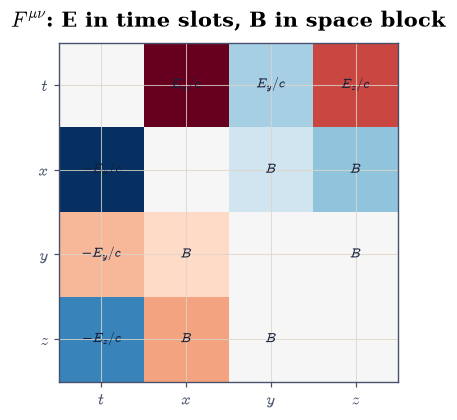
../../_images/cf762469d36fa59e8d5405ab98c0aa304338b14445a7903108584026b15bbe48.png — Fig. 286 The field tensor \(F^{\mu\nu}\) as a \(4\times4\) matrix (here normalised by its largest entry, diverging colour = sign). It is antisymmetric, so the diagonal is zero; the top row and left column (red/blue) hold the electric field \(E_i/c\), and the spatial \(3\times3\) block holds the magnetic field \(-\varepsilon^{ijk}B_k\). The six independent entries are exactly \(\mathbf E\) and \(\mathbf B\): one object, not two.#

Exercise 4 — Maxwell’s equations in covariant form (worked)#

Now the collapse. The two tensor equations Eq. 259 contain all four of Maxwell’s laws. The sourced equation \(\partial_\mu F^{\mu\nu}=\mu_0 J^\nu\) gives Gauss’s law for \(\nu=0\) and Ampère–Maxwell for \(\nu=i\); the Bianchi identity (the source-free pair) gives \(\nabla\cdot\mathbf B=0\) and Faraday. Eleven notebooks of separate laws, written in two lines.

What we check here is that unpacking, not a solution: the test field is an arbitrary smooth \(\mathbf E(t,\mathbf r)\), \(\mathbf B(t,\mathbf r)\) on a \(16^4\) grid over the unit spacetime box, and it need not satisfy Maxwell at all, because the identity between the tensor form and the 3-vector form holds field by field. Written out, the two components we test read \(\partial_\mu F^{\mu0}=-(\nabla\cdot\mathbf E)/c\) (Gauss) and \(\partial_\mu F^{\mu i}=(\nabla\times\mathbf B-\tfrac1{c^2}\partial_t\mathbf E)_i\) (Ampère–Maxwell).

Assemble \(F^{\mu\nu}\) on the 4-D grid: the same packing you wrote in Exercise 3, but with each entry now a whole array, so the \(4\times4\) is written out as a nested list rather than built by a call.
Write tensor_divergence(nu), forming \(\partial_\mu F^{\mu\nu}\) by differentiating each \(F^{\mu\nu}\) along its own \(x^\mu\) axis with numpy.gradient — and since \(x^0=ct\), the time derivative is \(\partial_0=\partial/\partial(ct)\) — then summing over \(\mu\). Write this one yourself — the implementation is the lesson: the whole content of a covariant equation is which index runs against which axis.
Confirm component by component that it equals the corresponding 3-vector operator, to finite-difference precision on the interior (the boundary nodes use one-sided differences, so they are excluded). The tensor equation is the 3-vector equations.

max |∂_μF^μ0 − (−∇·E/c)|        (Gauss)        = 8.48e-24
max |∂_μF^μx − (Ampère–Maxwell)_x|             = 2.22e-16

Validation 4#

✓  ∂_μF^μ0 = μ₀J⁰ reproduces Gauss's law (∇·E component-wise)   [max|Δ| = 8.4786e-24 (rtol=1e-06, atol=1e-09)]
✓  ∂_μF^μi = μ₀J^i reproduces Ampère–Maxwell (component-wise)   [max|Δ| = 2.22045e-16 (rtol=1e-06, atol=1e-09)]

True

Movement III — The unification: E and B mix#

Exercise 5 — Boosting the field tensor (worked)#

Because \(F^{\mu\nu}\) is a tensor, a change of frame acts on it by the boost on each index, \(F'^{\mu\nu}=\Lambda^\mu{}_\alpha\Lambda^\nu{}_\beta F^{\alpha\beta}\), i.e. \(F'=\Lambda F\Lambda^{\mathsf T}\) Eq. 260. Reading \(\mathbf E'\) and \(\mathbf B'\) out of the boosted tensor must reproduce the textbook transformation rules, with the parallel components unchanged and the perpendicular ones mixing \(\mathbf E\) and \(\mathbf B\). For a boost along \(x\) at \(v=0.6c\) those rules are \(E'_x=E_x\), \(E'_y=\gamma(E_y-vB_z)\), \(E'_z=\gamma(E_z+vB_y)\), and \(B'_x=B_x\), \(B'_y=\gamma(B_y+vE_z/c^2)\), \(B'_z=\gamma(B_z-vE_y/c^2)\) — derived by hand in the textbooks, one component at a time.

Boost the \(F^{\mu\nu}\) of Exercise 3 by contracting both indices with the lorentz_boost you wrote in Exercise 1: np.einsum('ma,nb,ab->mn', Λ, Λ, F), equivalently \(\Lambda F\Lambda^{\mathsf T}\).
Read \(\mathbf E'\) and \(\mathbf B'\) out of the result with your Exercise 3 extract_EB and check them against the closed-form rules above. Tensor algebra and the hand-derived formulas must agree to machine precision.

E' (tensor)  = [300000.    -80031.131 339937.737]
E' (formula) = [300000.    -80031.131 339937.737]
B' (tensor)  = [0.000000e+00 1.000346e-03 1.730714e-07]
B' (formula) = [0.000000e+00 1.000346e-03 1.730714e-07]

Validation 5#

✓  the boosted field tensor reproduces the E transformation law   [max|Δ| = 5.82077e-11 (rtol=1e-08, atol=1e-09)]
✓  the boosted field tensor reproduces the B transformation law   [max|Δ| = 2.1684e-19 (rtol=1e-08, atol=1e-09)]

True

Exercise 6 — Magnetism is electricity in another frame (worked)#

This is the volume’s deepest result. Take a pure electric field, \(\mathbf B=0\), the Coulomb field of a static charge, and look at it from a moving frame. A genuine magnetic field appears: \(\mathbf B'\neq0\) Eq. 260. There is no separate “magnetism” waiting in the wings; the magnetic field of a moving charge (§3.6) simply is its electric field, seen by an observer in motion (Fig. 287). The animation that closes the exercise sweeps the boost from \(0\) to \(0.9c\) and watches \(\mathbf B'\) grow from nothing as the frame speeds up, the unification set in motion.

Build the pure-\(E\) field tensor from \(\mathbf E=(0,10^5,0)\,\)V/m and \(\mathbf B=0\) with the field_tensor you wrote in Exercise 3, apply the perpendicular boost at \(v=0.6c\) with the same np.einsum('ma,nb,ab->mn', Λ, Λ, F) contraction as Exercise 5, and read \(\mathbf B'\) back out with your Exercise 3 extract_EB.
Show the magnetic field that emerges equals the closed form \(B'_z=-\gamma vE_y/c^2\).
Sweep \(\beta\) from \(0\) to \(0.9\), rebuilding \(\Lambda(\beta)\) each time with your Exercise 1 lorentz_boost, and animate \(E'_y\) and \(B'_z\) against \(\beta\) (Fig. 287).

lab frame:  E = [     0. 100000.      0.] V/m,  B = [0. 0. 0.] T
boosted (v=0.6c):  E' = [     0. 125000.      0.] V/m
                    B' = [ 0.       0.      -0.00025] T  ← appeared!
B'_z = −γvE_y/c² = -2.502e-04 T

Validation 6#

✓  a pure electric field acquires exactly B'_z = −γvE_y/c² under a boost — magnetism is relativity   [got -0.000250173 vs expected -0.000250173 (rtol=1e-08, atol=1e-09)]
✓  the boost generates no magnetic component along x or y (geometry of v × E)   [max|Δ| = 0 (rtol=1e-06, atol=1e-15)]

True

Fig. 287 Animation of the unification: a pure electric field (\(\mathbf E=E_0\hat{\mathbf y}\), \(\mathbf B=0\) in the lab) viewed from frames boosted along \(x\) at increasing speed. As \(\beta\) rises from \(0\) to \(0.9\), the electric field grows by \(\gamma\) and a magnetic field \(B'_z=-\gamma\beta E_0/c\) appears from nothing and strengthens. There is no separate magnetism: \(\mathbf B\) is what part of the one electromagnetic field looks like to a moving observer.#

Exercise 7 — The current-carrying wire, demystified (student)#

The most famous demonstration that magnetism is relativity is a neutral wire. In the lab it carries a current and exerts a magnetic force on a nearby moving charge. But in the charge’s own rest frame there is no motion of the charge to feel a magnetic force; instead, the wire’s positive and negative charge densities Lorentz-contract by different amounts, so the wire appears charged, and the same force arrives as an electric one. Two descriptions, one physics.

The model is positive ions at rest and electrons drifting at \(v_d\), each species with proper line density \(\lambda_0=10^{-8}\,\)C/m, so the wire is neutral in the lab; the test charge is \(q=1\,\)nC moving parallel to the wire at \(u=5\times10^5\,\)m/s, a distance \(r=0.02\,\)m away, and the drift is \(v_d=10^5\,\)m/s. Two facts from earlier do the work: the wire’s field \(B=\mu_0 I/2\pi r\) (§3.6) and the line charge’s field \(E=\lambda/2\pi\varepsilon_0 r\) (§3.3). One relativistic subtlety: a transverse force is not itself invariant — it picks up a factor \(\gamma_u\) between the lab and the charge’s rest frame, so the two forces are compared as \(F'/\gamma_u\) against \(F\).

In the lab, compute the current \(I=\lambda_0 v_d\) and the magnetic force \(F=quB\) on the test charge.
Transform to the charge’s rest frame: velocity-add the electron drift and the charge’s own motion, \(w_e=(v_d+u)/(1+v_du/c^2)\), and Lorentz-contract each species’ line density by its own \(\gamma\) — the ions now move at \(u\), the electrons at \(w_e\) — to get the net density \(\lambda_{\rm net}\), which is no longer zero.
Compute the rest-frame electric force \(F'=qE'\) with \(E'=\lambda_{\rm net}/2\pi\varepsilon_0 r\), and confirm \(F'/\gamma_u\) reproduces the lab’s magnetic force.

lab magnetic force      = 5.0000e-12 N
rest-frame electric force = -5.0000e-12 N
rest force / γ_u         = -5.0000e-12 N   (matches lab force)

Validation 7#

✓  the lab magnetic force equals the electric force in the charge's rest frame   [got -5e-12 vs expected 5e-12 (rtol=0.001, atol=1e-09)]

True

Movement IV — Invariants and structure#

Exercise 8 — The Lorentz invariants (worked)#

Although \(\mathbf E\) and \(\mathbf B\) each change from frame to frame, two combinations of them do not Eq. 262: the scalars \(\mathbf E\cdot\mathbf B\) and \(E^2-c^2B^2\), built from \(F_{\mu\nu}\widetilde F^{\mu\nu}\) and \(F_{\mu\nu}F^{\mu\nu}\), are the same in every frame. Whether a field is “more electric” or “more magnetic” is a matter of who is looking, but these two numbers are absolute, and they classify the field: a radiation field, for instance, has both invariants zero for every observer.

Write invariants(E, B), returning the pair \((\mathbf E\cdot\mathbf B,\;E^2-c^2B^2)\) as the dot product E @ B and the combination E @ E - c**2 * (B @ B).
Evaluate it on the lab-frame \(\mathbf E,\mathbf B\) of Exercise 3 and on the boosted \(\mathbf E',\mathbf B'\) of Exercise 5, and confirm both numbers are unchanged even though \(\mathbf E\) and \(\mathbf B\) themselves are not.

lab:     E·B = -8.0000e+01,   E²−c²B² = 1.2202e+11
boosted: E·B = -8.0000e+01,   E²−c²B² = 1.2202e+11

Validation 8#

✓  the two field invariants E·B and E²−c²B² are the same in all frames   [max|Δ| = 3.05176e-05 (rtol=1e-06, atol=1e-09)]

True

Exercise 9 — Gauge invariance as structure (worked)#

The gauge arc reaches its summit. Because \(F^{\mu\nu}=\partial^\mu A^\nu-\partial^\nu A^\mu\) and partial derivatives commute, adding the gradient of any scalar to the four-potential, \(A^\mu\to A^\mu+\partial^\mu\chi\) Eq. 261, changes nothing: \(\partial^\mu\partial^\nu\chi-\partial^\nu\partial^\mu\chi=0\). The gauge freedom that was a freedom in §3.6 and a tool in §3.8 is now seen as built into the very definition of the field, structure. And the Lorenz condition \(\partial_\mu A^\mu=0\), being a four-divergence, is manifestly Lorentz-invariant, where the Coulomb gauge \(\nabla\cdot\mathbf A=0\) is not.

The demonstration runs on the \((ct,x)\) sector alone, where a single component \(F^{tx}=\partial^tA^x-\partial^xA^t\) carries the whole story; with the signature \((-,+,+,+)\), raising the time index flips its sign, \(\partial^t=-\partial_{ct}\), while \(\partial^x=\partial_x\). The four-potential is \(A^0=\sin x\cos(ct)\), \(A^1=\cos x\sin(ct)\) and the gauge scalar is \(\chi=0.7\sin(x+ct)+0.3\cos 2x\), chosen for no reason at all — which is the point, since any \(\chi\) must leave \(F\) alone.

Write Fxt(A0, A1), building \(F^{tx}\) from a four-potential on the grid by differencing with numpy.gradient and raising both indices with the metric. Write this one yourself — the implementation is the lesson: the sign that the raised time index puts on \(\partial_{ct}\) is the whole content of “raising an index”.
Evaluate \(F^{tx}\) for that four-potential, then shift it by \(A^\mu\to A^\mu+\partial^\mu\chi\) (again via numpy.gradient, with the same raising rule), rebuild \(F^{tx}\), and confirm the two agree with np.allclose — here read off as the maximum difference on the interior, where the central differences are clean.

The arc closes: freedom (§3.6) → tool (§3.8) → structure (here) → physics (Vol VI, Aharonov–Bohm), rooted in the symmetry–conservation link of Noether (§2.2), where a global phase symmetry gives charge conservation and its local version is gauge symmetry itself.

max |F (after gauge change) − F (before)| = 9.77e-15  (identically 0)

Validation 9#

✓  F^μν is invariant under a gauge transformation A → A + ∂χ (gauge as structure)   [max|Δ| = 9.76996e-15 (rtol=1e-06, atol=1e-09)]

True

Exercise 10 — The stress–energy tensor: what the field carries#

One promise remains. §3.8 found that the field carries energy (the density \(u\) and the Poynting flux \(\mathbf S\)), and §3.10 spent that flux on radiation — but energy density, energy flux, momentum density, and momentum flux were four separate bookkeeping entries. Relativity refuses to keep them separate: they are the sixteen components of one symmetric tensor built from \(F^{\mu\nu}\) alone,

(263)#\[T^{\mu\nu} \;=\; \frac{1}{\mu_0}\left[F^{\mu\alpha}F^{\nu}{}_{\alpha} \;-\; \tfrac14\,\eta^{\mu\nu}F_{\alpha\beta}F^{\alpha\beta}\right],\]

whose slots are physics the volume already owns: \(T^{00}=u=\tfrac{\varepsilon_0}{2} (E^2+c^2B^2)\) is the energy density, \(T^{0i}=S_i/c\) is the Poynting flux, and the spatial block is \(T^{ij}=-\sigma_{ij}\), the (negative of the) Maxwell stress tensor. That last object is the working tool: \(\sigma_{ij}\) is built from the fields quadratically,

(264)#\[\sigma_{ij} \;=\; \varepsilon_0\!\left(E_iE_j-\tfrac12\delta_{ij}E^2\right) \;+\; \frac{1}{\mu_0}\!\left(B_iB_j-\tfrac12\delta_{ij}B^2\right), \qquad dF_i = \sigma_{ij}\,n_j\,dA,\]

and the force law on the right says something remarkable: the total electromagnetic force on everything inside a closed surface is a surface integral of the fields on that surface — no charges consulted, only the stress the field transmits across the boundary, tension along field lines and pressure across them. This exercise builds \(T^{\mu\nu}\), certifies every slot, watches it transform as the rank-2 tensor it is (the same law §3.16 tests on a material tensor, here obeyed by the field itself), and then earns the payoff: Coulomb’s force between two charges recovered from a stress integral that never touches Coulomb’s law.

Write stress_energy(F), evaluating Eq. 263 with two explicit metric placements: the inner contraction \(F^{\mu\alpha}F^{\nu}{}_{\alpha}\) as np.einsum("ma,ab,nb->mn", F, ETA, F) and the invariant scalar \(F_{\alpha\beta}F^{\alpha\beta}\) as np.einsum("am,bn,mn,ab->", ETA, ETA, F, F) (in this signature the matrix of \(\eta^{\mu\nu}\) equals that of \(\eta_{\mu\nu}\)). Write this one yourself — the implementation is the lesson: Exercise 9 raised one index; here the metric’s placement carries the whole definition.
Certify the slots on the lab field of Exercise 3, \(\mathbf E=(3,-1,2)\times10^5\) V/m and \(\mathbf B=(0,4,-2)\times10^{-4}\) T: \(T^{00}\) equals \(\tfrac{\varepsilon_0}{2}(E^2+c^2B^2)\), the row \(T^{0i}\) equals \((\mathbf E\times\mathbf B)/\mu_0 c\), and \(T^{\mu\nu}\) is symmetric and traceless (\(\eta_{\mu\nu}T^{\mu\nu}=0\) — the deep mark of a field whose quantum is massless).
Two frames, one tensor: transform \(T\) directly with the Exercise 1 boost, np.einsum("ma,nb,ab->mn", Λ, Λ, T), and compare against stress_energy of the boosted field tensor of Exercise 5 — the two routes must agree to machine precision. Then aim it at light: for the plane wave \(\mathbf E=E_0\hat{\mathbf y}\), \(\mathbf B=(E_0/c)\hat{\mathbf z}\) with \(E_0=10^4\) V/m travelling along \(+x\), confirm \(T^{xx}=T^{00}\) (radiation pressure on an absorber equals the energy density), and that chasing the wave at \(0.6c\) scales \(T^{00}\) by exactly \((1-\beta)/(1+\beta)=\tfrac14\) — each amplitude shrinks by the Doppler factor \(\sqrt{(1-\beta)/(1+\beta)}\), the energy density by its square.
The payoff. Two charges \(q=5\,\)nC sit at \(z=\pm a\) with \(a=10\,\)cm. Close a surface around the upper one: the midplane \(z=0\) (outward normal \(\hat{\mathbf n}=-\hat{\mathbf z}\)) plus a far hemisphere whose contribution dies as the integrand’s \(\rho^{-3}\) tail. On radii np.geomspace(1e-6, 100 * a, 4000), build \(\mathbf E\) as the broadcast vector sum of the two Coulomb fields, form \(\sigma_{zz}\) from Eq. 264, and integrate \(F_z=-\int\sigma_{zz}\,dA\) with np.trapezoid and the axisymmetric measure \(2\pi\rho\,d\rho\). Compare with Coulomb’s \(q^2/4\pi\varepsilon_0(2a)^2\), and confirm the truncation error falls as \((a/R)^2\) by repeating the integral cut at \(R=10a\).

T^00 = 6.993706e-01 J/m³   vs  ε0(E²+c²B²)/2 = 6.993706e-01
T^0i = [-0.15926512  0.15926512  0.31853025]  vs  S/c = [-0.15926512  0.15926512  0.31853025]
symmetric: True,   trace η_μν T^μν = -2.22e-16
tensor law: max|ΛΛT − T(ΛΛF)| = 2.22e-16
wave: T^xx/T^00 = 1.000000 (radiation pressure = u), boosted u'/u = 0.250000 vs (1−β)/(1+β) = 0.250000
stress integral F_z = 5.616112e-06 N   vs Coulomb 5.617220e-06 N (rel. 2.0e-04)
truncation: rel. error 2.0e-02 at R=10a vs 2.0e-04 at R=100a (ratio 100, the (a/R)² tail)

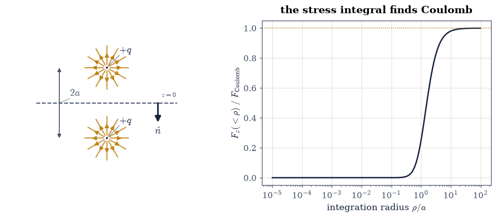
../../_images/95195b5b62f43d232f694a155636755014c97b4fd0c043bff6b6753bf4f91a92.png — Fig. 288 Coulomb’s force recovered from field stress alone. Left: two equal charges \(q\) at \(z=\pm a\) with radial field lines at equal angular spacing; the force on the upper charge is computed on a closed surface consisting of the midplane \(z=0\) (outward normal \(\hat{\mathbf n}=-\hat{\mathbf z}\), dashed) and a hemisphere pushed to infinity. Right: the running surface integral \(-\int\sigma_{zz}\,2\pi\rho\,d\rho\) out to radius \(\rho\), in units of the Coulomb force \(q^2/4\pi\varepsilon_0(2a)^2\); the integral climbs through the region \(\rho\sim a\) where the stress is concentrated and settles on 1 with a residual \((a/R)^2\) truncation tail. The field on the plane carries exactly the momentum flux that Newton’s third law requires.#

Validation 10#

✓  T^00 is the energy density ε0(E²+c²B²)/2 the volume already owns   [got 0.699371 vs expected 0.699371 (rtol=1e-12, atol=1e-09)]
✓  the row T^{0i} is the Poynting flux S/c   [max|Δ| = 5.55112e-17 (rtol=1e-12, atol=1e-09)]
✓  T^μν is symmetric and traceless (η_μν T^μν = 0), as a massless field demands   [trace/scale = 3.2e-16]
✓  T transforms as a rank-2 tensor: boosting T equals rebuilding T from the boosted F   [max|Δ| = 2.22045e-16 (rtol=1e-09, atol=6.99371e-13)]
✓  for a plane wave the momentum flux along propagation equals the energy density (radiation pressure = u)   [got 0.000885419 vs expected 0.000885419 (rtol=1e-12, atol=1e-09)]
✓  chasing the wave at 0.6c scales its energy density by the squared Doppler factor 1/4   [got 0.25 vs expected 0.25 (rtol=1e-09, atol=1e-09)]
✓  on the midplane the two charges' E_z cancels to machine precision (measured, not imposed)   [max|E_z|/max|E_ρ| = 0.0e+00]
✓  the surface integral of Maxwell stress over the midplane reproduces Coulomb's force without consulting Coulomb's law   [got 5.61611e-06 vs expected 5.61722e-06 (rtol=0.001, atol=1e-09)]
✓  and the truncation error falls as (a/R)²: cutting the plane at 10a costs about 100× the error of cutting at 100a   [2.0e-02 / 2.0e-04 = 100]

True

Exercise 11 — What the volume built#

Stand at the summit and look back. The volume opened with a single static charge and the question of what it does to the space around it (§3.1). It found a field, then a potential, then a local law (Gauss, §3.3); it added magnetism (§3.6), coupled the two through induction (§3.7), and closed the set with the displacement current into Maxwell’s equations and the discovery that light is an electromagnetic wave (§3.8). It confined those waves (§3.9), found what produces them (§3.10), and met them again as circuits (§3.11). And here, at the end, all of it, eleven notebooks of separate laws, collapses into two tensor equations for a single object \(F^{\mu\nu}\) in a four-dimensional spacetime. Electrodynamics is revealed as one relativistic field theory, the first and the exemplar of classical field theory.

The crisis that drove us, “\(c\) relative to what?”, is resolved: there is no preferred frame, \(\mathbf E\) and \(\mathbf B\) are one object, and the laws read the same for every observer. The road continues to special relativity in full (Vol IV), to quantum electrodynamics where gauge invariance becomes physics (Vol VI), and to field theory beyond. The volume began by asking what a charge does to the space around it, and ends by finding that space, time, electricity, and magnetism are one structure.

Confirm the summit numerically in one line: the same field configuration, viewed in the lab and in the boosted frame of Exercise 5, has different \(\mathbf E\) and \(\mathbf B\) but identical invariants and an identical, antisymmetric \(F^{\mu\nu}\) structure — the single object underneath the two appearances.

E and B differ between frames; the invariants and the tensor structure do not.
one electromagnetic field, seen two ways: True
Volume III complete: from a static charge to a single relativistic field theory.

Validation 11#

✓  one electromagnetic field: frame-independent invariants and an antisymmetric F^μν

True

Notebook summary#

Spacetime and four-vectors. The boost \(\Lambda(0.6c)\) preserves the interval \(s^2=\eta_{\mu\nu}x^\mu x^\nu\) and maps light rays to light rays (\(c\) invariant); the four-velocity has norm \(u^\mu u_\mu=-c^2\), and the Lorenz gauge is the single four-divergence \(\partial_\mu A^\mu=0\).
The field tensor. \(\mathbf E\) and \(\mathbf B\) are the six components of one antisymmetric \(F^{\mu\nu}\) Eq. 258 (round-tripped exactly), and Maxwell’s four equations are the two tensor lines \(\partial_\mu F^{\mu\nu}=\mu_0 J^\nu\) and the Bianchi identity, verified component-by-component against \(\nabla\cdot\mathbf E\) and \(\nabla\times\mathbf B-\tfrac1{c^2}\partial_t\mathbf E\).
The unification. Boosting \(F^{\mu\nu}\) reproduces the \(\mathbf E,\mathbf B\) transformation laws to machine precision; a pure electric field acquires a magnetic one under a boost (\(B'_z=-\gamma vE_y/c^2\), animated), and the current-carrying wire’s magnetic force is an electric force in the charge’s frame. Magnetism is electricity in motion.
Invariants and structure. \(\mathbf E\cdot\mathbf B\) and \(E^2-c^2B^2\) are the same in every frame; \(F^{\mu\nu}=\partial^\mu A^\nu-\partial^\nu A^\mu\) is manifestly gauge-invariant, closing the arc freedom (§3.6) → tool (§3.8) → structure (here) → physics (Vol VI), rooted in Noether (§2.2).
What the field carries. The stress–energy tensor \(T^{\mu\nu}\) Eq. 263 holds the volume’s energy bookkeeping in one symmetric, traceless object: \(T^{00}=u\), \(T^{0i}=S_i/c\), spatial block \(-\sigma_{ij}\). It transforms as a rank-2 tensor to machine precision; a plane wave’s radiation pressure equals its energy density, and chasing it at \(0.6c\) scales \(u\) by exactly \((1-\beta)/(1+\beta)=\tfrac14\); and the Maxwell stress integrated over a midplane reproduces Coulomb’s force between two charges to \(2\times10^{-4}\) without consulting Coulomb’s law. From a static charge (§3.1) to one relativistic field theory: Volume III complete.

Outlook#

Special relativity in full (Vol IV). Kinematics, dynamics, \(E=mc^2\), and the spacetime geometry developed here only as far as electrodynamics required.
The stress–energy tensor as a source. Exercise 10 built \(T^{\mu\nu}\) and watched it transform; in general relativity it stands on the right-hand side of Einstein’s equations, the object that curves spacetime — the role the GR capstone (§4.8) gives it. Still undelivered here: the field’s angular momentum (the moment of \(T^{0i}\)), and the delicate bookkeeping of field momentum in matter (the Abraham–Minkowski question).
Relativistic radiation. The Liénard–Wiechert potentials extend the radiation of §3.10 to fast charges, giving synchrotron light and the relativistic beaming of accelerators.
Gauge theory and the Standard Model. Promoting the global phase symmetry of Noether (§2.2) to a local one is electromagnetism; generalising the group leads to Yang–Mills theory and the Standard Model, far beyond this course’s arc.
Quantum electrodynamics (Vol VI). Gauge invariance becomes physical in the Aharonov–Bohm effect, and minimal coupling weds the four-potential to the quantum particle, where this volume’s structure becomes the language of modern physics.

Take this notebook with you

Use the download button (↓) in the toolbar above to save this notebook and run it yourself. The published notebooks ship without worked solutions; if you would like the reference solutions — to teach from or to check your own work — get in touch: hello@ramador.me.