


5.18 Nucleation: The Critical Droplet and the Metastable Lifetime#
Notebook overview#
A phase can be wrong and still be stable. Water held at \(-5\,^\circ\)C in a clean, still glass stays liquid; water heated past \(100\,^\circ\)C in a smooth mug in a microwave stays liquid, and then, when something finally disturbs it, boils all at once and all over the counter. In between the two states there is no continuous downhill path: the system has to build a piece of the new phase before the new phase can lower the free energy at all, and building that piece costs surface. That cost is a barrier, the barrier makes the wrong phase long-lived, and the whole subject of nucleation is the arithmetic of that one competition.
§5.15 promised this notebook almost word for word: the metastable strips between binodal and spinodal decay by rare fluctuations, with a free-energy barrier and Arrhenius kinetics. We deliver it in the model where every ingredient can be computed exactly rather than modelled: the two-dimensional Ising magnet of §5.10, with one thing added. That notebook had no external field, and without a field the two ordered states are exactly degenerate, so neither is metastable. Adding \(-H\sum_i\sigma_i\) to the energy tilts them apart, and then a magnet prepared in the wrong well behaves exactly like superheated water: it waits, it looks perfectly ordinary while it waits, and then it goes.
What we build: the field into the Metropolis update (three lines, and one of them is the physics);
the metastable lifetime and its distribution; cluster identification with scipy.ndimage.label,
which this course has never needed before; the critical droplet, measured twice, once by seeding
droplets and asking which ones survive and once from the free energy read off cluster statistics;
and the field dependence of the lifetime, which classical nucleation theory says is
\(\ln\tau\propto1/|H|\) in two dimensions. Every prediction is checked against Onsager’s exact
interfacial tension and spontaneous magnetization, so the comparison is with real numbers and not
with a fitted curve.
How to read the checks. Each exercise closes with a
validatecall against an independent fact: that the field enters the energy difference exactly as the Hamiltonian says and reduces to §5.10 when it is switched off; that the lifetime is exponentially distributed, as a single rare event must be; that the labelled clusters of a hand-built lattice are the ones we drew; that the critical droplet size scales as \(1/|H|\); that the free-energy cost of a one-spin cluster is exactly \(8J\); that the lifetime obeys \(\ln\tau \propto1/|H|\) with the Onsager coefficient. Monte Carlo lifetimes are random variables, so every check here is a check on a distribution or on many seeded runs, never on one realisation. A ✓ is strong evidence; a ✗ is a prompt to locate the discrepancy.Scope, and an honest boundary. Three limits are drawn deliberately, and each one is drawn in the open. (1) The rate prefactor is out of scope. We compute the barrier — the critical droplet, its free energy, and the exponential it puts into the lifetime — and we do not compute the attempt frequency in front of that exponential. Getting it right means writing a Fokker–Planck equation for the probability flux in cluster-size space, which is the Becker–Döring theory and its Zeldovich factor; Landau and Lifshitz carry it out in Physical Kinetics §99 [LP81], importing the barrier wholesale from equilibrium statistical mechanics exactly as we do here. Both of the teaching treatments this notebook follows, Exercise 11.4 of [Set21] and Chapter 5 of [GTC07], stop in the same place. (2) No umbrella sampling and no forward-flux sampling. We run at driving strong enough that nucleation happens unaided within a plain Metropolis run. That is a scope choice, not an oversight: §5.11 assigns rare-event and free-energy methods outward to molecular-simulation courses, and Exercise 5 shows precisely where the unaided histogram runs out of samples and what an enhanced-sampling method would be for. (3) Nucleation is not coarsening. Quenching in temperature through \(T_c\), which §5.10 already animates, gives domain coarsening out of an unstable symmetric state; flipping the field at fixed temperature gives nucleation out of a metastable one. Exercise 8 puts them side by side and measures the difference rather than asserting it. Cross-reference §5.10 (the model and the sampler), §5.8 (Metropolis), §5.7 (free energy and convexity), §5.15 (the metastable strip this delivers), §5.17 (error bars on correlated runs), and E.3 (the honest-boundary discipline).
Theory in brief#
The Ising model acquires a field#
§5.10 worked with spins \(\sigma_i=\pm1\) on a square lattice that pay an energy penalty for disagreeing with their neighbours, and with nothing else. A real magnet also sits in an applied field, which couples to each spin separately and prefers one direction outright, so the energy gains a second term,
We keep \(J=k=1\) throughout, so temperature and field are measured in units of \(J\) and the critical temperature is still Onsager’s \(T_c=2/\ln(1+\sqrt2)\approx2.269\). The field term destroys the \(\mathbb{Z}_2\) symmetry that was the whole subject of §5.10: “all up” and “all down” are no longer degenerate, and at \(H>0\) the up state is the true equilibrium while the down state is merely a local minimum of the free energy. That asymmetry is the entire point. The lattice, parked in the local minimum, is metastable, and the question of how long it stays there is the question of this notebook.
Metropolis needs only the energy change on flipping one spin. Flipping \(\sigma_i\) reverses both its bond energy and its field energy, so from Eq. 477
which is §5.10 with \(H\) added inside the bracket, beside the neighbour sum. That placement is the physics: the field acts on the flipping spin like one more neighbour, of adjustable and non-integer strength. Everything else about the sampler is unchanged, which is why the update below can be checked against the old one by switching \(H\) off.
Why a metastable phase has to wait#
Suppose the field points down, \(H<0\), but the lattice is still up. Converting the whole lattice would lower the free energy, and yet nothing happens for a long time, because the conversion cannot proceed a spin at a time. Turn over a single spin and it is surrounded by four disagreeing neighbours: the bond cost \(8J\) swamps the field gain \(2|H|\), and it flips straight back. Only a compact region of down spins has a favourable surface-to-area ratio, and only if it is large enough.
That is classical nucleation theory in one sentence, and its arithmetic is a competition between a perimeter and an area. Write \(\sigma\) for the interfacial free energy per unit length of the wall between the two phases, and \(\Delta f\) for the free-energy difference per site between the metastable phase and the stable one. A circular droplet of the stable phase of radius \(R\) embedded in the metastable phase then costs
where the second relation is just bookkeeping: flipping one site from the metastable orientation to the stable one changes its field energy by \(2|H|\), and the phase is magnetized to \(m_s\) rather than fully, so per site the gain is \(2|H|m_s\). State the convention, because the literature uses several: our \(\Delta f\) is the free-energy difference per site, with the factor of two from \(\sigma\to-\sigma\) already inside it. Writers who define \(\Delta f=|H|m_s\) report a critical radius twice ours, and writers who work with a droplet diameter rather than a radius report another factor of two on top. The physics is in the ratio \(\sigma/\Delta f\), which is the only length the problem contains.
The first term of Eq. 479 grows linearly and the second quadratically, so \(\Delta F\) rises, turns over, and falls. Setting \(\mathrm{d}\Delta F/\mathrm{d}R=0\) gives the critical droplet, and evaluating \(\Delta F\) there gives the barrier,
A droplet smaller than \(R_c\) shrinks, because shedding perimeter saves more than shedding area costs; a droplet larger than \(R_c\) grows without limit. The critical droplet is a saddle, not a minimum: it is unstable in the one direction that matters, which is exactly why the reader can find it by asking which seeded droplets survive.
On a square lattice a square droplet is at least as natural as a round one, and it is what a seeded configuration will actually look like. Repeating the algebra with a square of side \(\ell\), perimeter \(4\ell\) and area \(\ell^2\),
so the critical square has half-side \(\sigma/\Delta f\), exactly the critical circle’s radius, and a barrier larger by \(4/\pi\). The two conventions bracket the truth. The genuine equilibrium shape is neither, because the interfacial tension of the Ising model depends on the angle the wall makes with the lattice; the shape that minimises \(\oint\sigma(\theta)\,\mathrm{d}s\) at fixed area is the Wulff shape, a rounded square. We will keep both bracketing forms and report where the measurement falls between them, which is more honest than choosing one and pretending.
The two numbers we need, exactly#
What makes the Ising model the right laboratory is that both quantities in Eq. 479 are known in closed form on the square lattice, from the same exact solution that gave §5.10 its \(T_c\). The spontaneous magnetization is Onsager’s and Yang’s, and the interfacial free energy per unit length along a lattice axis is Onsager’s,
Neither is derived here — they are quoted results, on the same footing as \(T_c\) in §5.10, and the exact solution behind them is developed in the Materials Modelling course and in Chapter 8 of [Set21]. Both are worth a moment’s reading, though. The tension tends to \(2J\) as \(T\to0\), which is exactly the bond cost of one unit length of straight domain wall, and it vanishes at \(T_c\), where the two phases stop being distinguishable and a wall between them costs nothing. At our working temperature \(T=1.5\) they take the values \(m_s=0.9865\) and \(\sigma=1.1901\), so the only length in the problem is \(\sigma/\Delta f=0.6031/|H|\) lattice spacings: at \(|H|=0.25\) the critical droplet is about two and a half spacings across. Small droplets are what a lattice this size can afford, and the sharp-interface picture of Eq. 479 is being asked to describe an object only a few interface widths wide. That is a real limitation and we will see it in the numbers.
From the barrier to the lifetime#
The metastable state decays when a fluctuation carries some region over the saddle. Because the barrier is large compared with \(kT\), that is a rare event, and rare events governed by a barrier obey an Arrhenius law: the rate per site is \(I=A\,\mathrm{e}^{-\Delta F_c/kT}\), the whole lattice offers \(N=L^2\) independent places for it to happen, and the lifetime is the reciprocal of the total rate,
where the second form follows by putting \(\Delta f=2|H|m_s\) into Eq. 480 or Eq. 481. The prediction is sharp and unusual: the logarithm of the lifetime is linear in the inverse field, with a slope fixed by Onsager’s two numbers and nothing else. At \(T=1.5\) it is \(\Xi=1.503\) for the circular convention and \(1.914\) for the square one. Exercise 7 measures it.
The prefactor \(A\) is a different matter. It is not a constant — it carries its own field dependence and its own temperature dependence, and computing it means asking how probability flows through the saddle region in cluster-size space rather than merely how improbable the saddle is. That calculation is Becker–Döring kinetics with Zeldovich’s correction for the recrossing of a flat barrier top, and it is where a nucleation notebook turns into a physical kinetics course. We stop at the exponential, say so, and point to Landau and Lifshitz, Physical Kinetics §99 for the rest. One consequence is worth carrying: because \(A\) depends on \(|H|\) too, the apparent slope of \(\ln\tau\) against \(1/|H|\) over a narrow window is the barrier coefficient \(\Xi\) plus a prefactor contribution, and separating them needs a range of fields we cannot afford.
Where the single-droplet picture holds#
One more piece of theory, and it is the piece the textbooks leave out. Everything above assumed that decay proceeds by one critical droplet, which then grows to fill the system. Whether that is true depends on the race between the waiting time \(\tau\) for a droplet to appear and the time \(L/v\) for a droplet to sweep across the lattice at its growth velocity \(v\). If \(\tau\gg L/v\) the first droplet takes over and the decay is a single stochastic event; if \(\tau\lesssim L/v\) many droplets nucleate independently and the decay is a smooth deterministic filling. Rikvold, Tomita, Miyashita and Sides [RTMS94] map this out and find four distinct field regimes for the metastable lifetime, of which the clean textbook story occupies one. The crossover field out of the single-droplet regime shrinks only as \(1/\ln L\), so it cannot be escaped by making the system a little smaller.
The two regimes leave different fingerprints, and both are cheap to measure. In the single-droplet regime the decay is a Poisson process, so the lifetime is exponentially distributed and its standard deviation equals its mean; and because every site is an independent candidate, \(\tau\propto L^{-2}\), so \(\tau L^{2}\) is a constant. In the multi-droplet regime the lifetime is an average over many independent nucleation events, so its distribution is narrow and \(\tau\) stops depending on \(L\). Exercise 6 measures both fingerprints across lattice sizes and finds where the crossover sits — including at the parameters the textbooks use.
Setup#
Units are those of §5.10: \(J=k=1\), temperature and field in units of \(J\), lengths in lattice spacings, time in Metropolis sweeps. The data are the working state point (\(T=1.5\), \(|H|=0.25\), \(L=24\)), the series palette with the two-colour map that renders a spin lattice, and the three exact results quoted from Onsager’s solution — the critical temperature, the spontaneous magnetization, and the interfacial tension of Eq. 482. Those last two are closed forms this notebook is handed rather than machinery it builds; they are the specimen every measurement is compared against. The instruments are the checkerboard mask builder and a snapshot-plotting scaffold, plus the zero-field Metropolis sweep of §5.10, restated here because Exercise 1 certifies its own field-carrying replacement against it.
This notebook’s own machinery is not here. The field in the energy and in the acceptance rule is Exercise 1, the metastable driver and the lifetime are Exercise 2, cluster identification is Exercise 3, and the droplet-survival estimator is Exercise 4. Every run below is driven by the routines built in those exercises.
The Setup below holds this notebook’s data and instruments — nothing you are asked to build. It is collapsed so the building stays yours; expand it whenever you want the details.
Exercise 1 — The field in the energy, and in the acceptance rule (student)#
Everything this notebook does rests on one modification of the sampler of §5.10, so it is worth getting exactly right and worth certifying properly. The energy is Eq. 477, \(E=-J\sum_{\langle ij\rangle}\sigma_i\sigma_j-H\sum_i\sigma_i\) with \(J=1\) and periodic boundaries, and the energy change on flipping the single spin \(\sigma_i\) is Eq. 478, \(\Delta E_i=2\sigma_i(\sum_{j\in\langle i\rangle}\sigma_j+H)\): the field sits inside the bracket, added to the neighbour sum, because it acts on the flipping spin exactly as one more neighbour would (Fig. 501). Writing it outside — \(2\sigma_i\sum_j\sigma_j+H\) — is the natural slip, and it is invisible at \(H=0\), so the check below is built to catch it at \(H\ne0\) rather than to reassure at \(H=0\).
The certification has three parts because there are three things that can be wrong, and each part is chosen so that it can actually fail. First, the bracket. Rather than trusting Eq. 478, compute \(\Delta E_i\) the slow honest way for every site of a generic random \(8\times8\) lattice at the deliberately non-round field \(H=0.37\): evaluate the total energy, flip site \(i\), evaluate it again, take the difference, and compare with the formula. A misplaced field term disagrees at every site. Second, the reduction. At \(H=0\) the new sweep must be the old sweep, not merely similar to it: driven from the same seed on the same starting lattice, the two consume their random numbers in the same order and must produce bitwise identical configurations. Run that comparison on a random \(16\times16\) lattice at \(T=2.5\), hot enough that a large fraction of sites flips every sweep, so agreement is a real coincidence and not the trivial agreement of two lattices that never move. Third, the converse: at \(H=0.4\) on the same stream the two must differ, which is what shows the field term is alive rather than multiplied by zero somewhere.
Part a) Write ising_energy(s, h) returning the total energy of Eq. 477 for
a lattice s at field h, counting each bond once (sum \(s\cdot\)numpy.roll(s,-1,axis) over the
two axes, which visits every periodic bond exactly once) and subtracting h * s.sum().
Part b) Write ising_sweep_field(s, beta, h, rng, masks), one in-place Metropolis sweep at
field h: form the neighbour sum with the four numpy.roll shifts as in
§5.10, build dE from Eq. 478, and accept with
rng.random(s.shape) < np.exp(-beta*dE) restricted to each checkerboard mask in turn.
Write this one yourself — the implementation is the lesson: the field’s place inside the
bracket is the only new physics in the notebook, and it is the one line a library call would
hide.
Part c) Certify the two of them by the three tests above, and report the largest formula-versus-brute-force discrepancy over the 64 sites, whether the \(H=0\) lattices are identical, and the fraction of sites at which the \(H=0.4\) lattices differ.
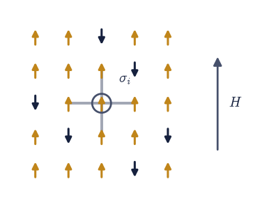
Fig. 501 Where the field enters a single-spin flip. A patch of the square lattice with up spins in amber and down spins in ink, matching the snapshots elsewhere in this notebook; the ringed site \(i\) is the candidate for flipping and the four highlighted bonds are the ones whose energy changes with it. Flipping \(\sigma_i\) reverses each of those four bond energies, giving the neighbour-sum term \(2J\sigma_i\sum_{j}\sigma_j\), and reverses the field energy of that one site, giving the extra \(2H\sigma_i\); the two combine into the single bracket of Eq. 2, so the field acts on the flipping spin exactly like one further neighbour of adjustable strength \(H\).#
the field in the energy difference, eq-nuc-dE  (T = 2.5, 30 sweeps):
  formula vs brute force over all 64 sites at h = 0.37: max gap = 8.88e-16
  h = 0 reduces to the §5.10 sweep, bitwise: True   (that run moved 52% of the sites, so the match is not trivial)
  h = 0.4 on the same stream differs at 86% of sites — the field is live
Validation 1#
✓ the field enters the flip energy inside the bracket, dE = 2 sigma (sum_nbr + H): the formula matches a brute-force energy difference at every site, the sweep reduces bitwise to the zero-field sweep of §5.10 on a configuration that moves, and it genuinely differs once the field is switched on [max |dE gap| = 8.9e-16, sites moved = 0.52, sites differing at h=0.4 = 0.86]
True
Exercise 2 — A magnet in the wrong well, and how long it stays there (student)#
Now the experiment the whole notebook is about. Prepare a lattice deep in the ordered phase at \(T=1.5\) with the field pointing up, \(H=+0.25\), so the magnetization settles near \(+m_s=+0.9865\) and the configuration is a placid sea of up spins. Then reverse the field to \(H=-0.25\) without touching the temperature. Nothing about the lattice changes at that instant, but everything about its status does: the state it is in has become the wrong one, higher in free energy than the down state by \(\Delta f=2|H|m_s\) per site, and the only thing keeping it there is the droplet barrier of Eq. 480.
What follows is the signature of metastability, and it looks nothing like a relaxation. The magnetization does not drift downward. It sits at \(+m_s\), indistinguishable from equilibrium, for a while that varies wildly from run to run, and then it collapses to \(-m_s\) over a few tens of sweeps (Fig. 502). Define the lifetime \(\tau\) as the first sweep at which \(m\) crosses zero, the standard choice in both [GTC07] and Exercise 11.4 of [Set21], and the collapse is fast enough that the answer barely depends on where the threshold is put.
The distribution of \(\tau\) over many seeds is the first real physics here, and it is a stronger statement than the mean. If the decay is triggered by a single rare event that is equally likely in every sweep and carries no memory of how long the system has already waited, then \(\tau\) is exponentially distributed: the survival probability is
whose standard deviation equals its mean and whose logarithm is a straight line against \(t\). That is a genuine test of the nucleation picture, not a restatement of it: a decay proceeding by steady growth from the moment of the flip, or by many simultaneous events, would give a narrow distribution instead. So the check is on the shape of the histogram over 150 seeded runs, never on any one of them.
Part a) Write metastable_run(L, T, h, rng, n_sweeps, burn=60), which allocates an all-up
\(L\times L\) lattice, equilibrates it for burn sweeps at field \(+h\) with the
ising_sweep_field of Exercise 1, then runs n_sweeps sweeps at field \(-h\) and returns the
per-sweep magnetization \(m=\frac1N\sum_i\sigma_i\) together with the final configuration.
Part b) Write lifetime(L, T, h, seed, max_sweeps), which performs the same preparation from
numpy.random.default_rng(seed) and returns the first sweep index after the reversal at which
\(m<0\), or max_sweeps if the run survives that long.
Part c) Plot six magnetization traces at \(L=32\), \(|H|=0.25\), \(T=1.5\) over 1200 sweeps, with the two equilibrium levels \(\pm m_s\) marked, and confirm by eye that the waiting time and not the collapse is what varies.
Part d) Collect 150 lifetimes at \(L=24\), \(|H|=0.25\), \(T=1.5\) from seeds \(500\ldots649\) with
max_sweeps=20000; report the mean, the median, and the ratio of standard deviation to mean; and
fit \(\ln P(\tau>t)\) against \(t\) over the lower 85% of the sorted lifetimes (numpy.polyfit,
degree 1) to test Eq. 484. For an exponential the ratio is \(1\) and the median is
\(\ln2\approx0.693\) times the mean.
metastable decay at T = 1.5, |H| = 0.25, L = 24  (150 seeded runs):
  mean lifetime             652.1 sweeps
  median lifetime           482.5 sweeps   (an exponential gives 452.0)
  std / mean                0.879          (an exponential gives 1)
  log-survival fit       slope -0.00159 vs -1/tau = -0.00153,  R^2 = 0.9922
  runs censored at 20000 sweeps: 0
Validation 2#
✓ the metastable lifetime is exponentially distributed over 150 seeded runs — the decay is a memoryless rare event, not a steady relaxation [std/mean = 0.88 (exponential: 1), log-survival R^2 = 0.992]
True
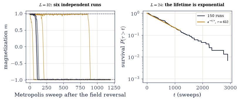
Fig. 502 Metastable decay of a \(32\times32\) Ising magnet at \(T=1.5\) after the field is reversed from \(H=+0.25\) to \(H=-0.25\) at sweep zero. Left: six magnetization traces from independent seeds, with the two equilibrium levels \(\pm m_s=\pm0.9865\) dashed; each run sits at the wrong equilibrium for a waiting time that varies by an order of magnitude between seeds and then falls to the right one within a few tens of sweeps, so what is random is the wait and not the collapse. Right: the survival probability \(P(\tau>t)\) of 150 lifetimes measured at \(L=24\) under the same conditions, on a logarithmic axis, against the exponential of Eq. 8 with the measured mean (amber); a straight line here says the decay is triggered by a single memoryless event whose probability per sweep does not depend on how long the system has already waited.#
Exercise 3 — Finding the droplets (student)#
The traces of Exercise 2 say when the decay happens and say nothing at all about what happens,
and everything that follows needs the configurations rather than their average. A droplet is a
connected region of minority spins, so we need to be able to take a lattice and hand back a list
of its connected regions with their sizes. That is a standard image-processing operation and this
course has not needed it once in seventeen notebooks: scipy.ndimage.label walks a boolean array
and assigns every connected component an integer, and numpy.bincount on the result counts them.
Connectivity has to be declared, and the declaration is physics rather than convention: two sites
belong to the same droplet when they are nearest neighbours, because those are the pairs the
Hamiltonian Eq. 477 couples, so the structuring element is the four-neighbour
cross NEIGHBOURS of the Setup and not the eight-neighbour square that scipy uses by default.
One honest limitation comes with the tool. The lattice is periodic but scipy.ndimage.label is
not: a droplet straddling the left and right edges is returned as two clusters rather than one.
For everything this notebook measures that is harmless, because the clusters we care about are
the small subcritical ones fluctuating inside the metastable phase, and by the time a droplet is
wide enough to wrap around the lattice it has long since crossed the barrier and stopped being a
droplet. Rather than assume the harm is small, Part c) measures it: the fraction of clusters that
touch any edge of the lattice at all is an upper bound on the fraction that could be mis-split.
Part a) Write label_clusters(s, value) which labels the connected components of
s == value with scipy.ndimage.label(..., structure=NEIGHBOURS) and returns the label array
together with a numpy.bincount-derived array of cluster sizes with the background dropped.
Part b) Certify it on the \(6\times6\) configuration below, which is all up except for a deliberate arrangement of down spins: an isolated site at \((0,0)\), a horizontal pair at \((2,3),(2,4)\), a four-site L at \((4,1),(5,1),(5,2),(5,3)\), and a diagonal touching pair at \((0,4),(1,5)\) that four-connectivity must count as two clusters and eight-connectivity would wrongly merge into one. The sorted sizes must come back as \([1,1,1,2,4]\).
Part c) Take a snapshot of the metastable phase at \(L=64\), \(T=1.5\), \(H=-0.25\) after 40 sweeps
using the metastable_run of Exercise 2, label its down-spin clusters, and report how many there
are, the size of the largest, the mean size, and the fraction touching an edge. The lattice is
still magnetized at \(m\approx+0.95\) at that moment, so what the labels find are fluctuations
inside the metastable phase and not the aftermath of a decay.
cluster labelling with scipy.ndimage.label and four-connectivity:
  hand-built 6x6 lattice: sorted cluster sizes = [1, 1, 1, 2, 4]   (expected [1, 1, 1, 2, 4])
  metastable snapshot, L = 64, 40 sweeps at H = -0.25:
    35 down clusters, largest 18 sites, mean 2.71, lattice still at m = +0.954
    fraction touching a lattice edge: 0.057 — an upper bound on those the non-periodic labelling could split
Validation 3#
✓ the four-connected labelling returns exactly the clusters drawn on the hand-built lattice, keeping the corner-touching pair apart, and the boundary-splitting error of the non-periodic labeller is bounded below 20% [sizes = [1, 1, 1, 2, 4], edge fraction = 0.057]
True
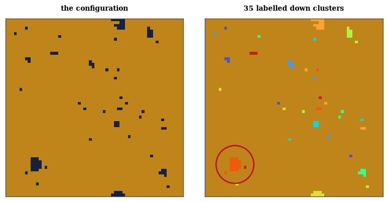
Fig. 503 Droplets in the metastable phase, found by labelling. Left: a \(64\times64\) configuration 40 sweeps after the field was reversed to \(H=-0.25\) at \(T=1.5\), still magnetized at \(m=+0.95\), with up spins in amber and down spins in ink; the metastable phase is not quiet but speckled with down-spin fluctuations, the largest of them close to the critical size Eq. 4 predicts and none of them yet committed to growing. Right: the same configuration with each four-connected down cluster given its own colour and the largest one ringed in red, the object whose size distribution Exercise 5 turns into a free energy. Clusters are counted with a nearest-neighbour structuring element, so two sites meeting only at a corner stay separate, and the labelling is not periodic, so a cluster wrapping the boundary would be split.#
The decay, watched#
The traces and the cluster counts describe the same event from two sides, and the event itself is worth seeing. What follows is a single \(64\times64\) run at \(T=1.5\) after the field is reversed to \(H=-0.25\), snapshotted every second sweep (Fig. 504). The metastable phase fluctuates without going anywhere, small dark patches appearing and vanishing; then one of them does not vanish, and from that moment the outcome is decided. Watch for one thing in particular, because Exercise 6 will make it quantitative: whether the lattice is taken over by one droplet or by several that appear at about the same time and then run into each other.
decay animation: 64 frames over 126 sweeps, m from +0.993 to -0.885
Fig. 504 Animation of a metastable decay: a \(64\times64\) Ising magnet at \(T=1.5\), prepared in equilibrium at \(H=+0.25\) and then held at \(H=-0.25\) from sweep zero, with up spins in amber and down spins in ink. Nothing happens for many sweeps beyond a speckle of subcritical fluctuations that appear and die; then one droplet reaches the critical size of Eq. 4 and grows without limit, its wall sweeping across the lattice at a roughly constant velocity until the whole system has converted. The title carries the sweep count and the instantaneous magnetization \(m\), whose fall to \(-m_s\) is the collapse seen in Fig. 3.#
Validation 3b#
✓ the animated run begins at the metastable equilibrium, holds there through the first third of its life, and then converts completely — a waiting time followed by a collapse, not a drift [m: +0.993 -> -0.885]
True
Exercise 4 — The critical droplet, route one: which droplets survive (student)#
The critical droplet of Eq. 480 is defined by an instability, and an instability can be measured directly rather than inferred. Plant a droplet of the stable phase by hand, of a size we choose, in an otherwise metastable lattice; let the dynamics run; and record whether it grew or died. Small droplets almost always die and large ones almost always grow, so the probability of growth rises from zero to one as the seeded size increases, and the size at which it passes \(\tfrac12\) is the critical droplet as the dynamics itself defines it. This is the committor construction, and it needs no free-energy calculation at all.
Seed squares rather than discs. A disc rasterized onto a lattice has a ragged perimeter whose length jumps about as the radius changes, so its survival probability is not even monotonic in the radius; a square of side \(\ell\) has perimeter exactly \(4\ell\), which is why Eq. 481 was worth writing down. The prediction to test is therefore \(\ell_c=2\sigma/\Delta f\) with \(\Delta f=2|H|m_s\), which at \(T=1.5\) is \(\ell_c=1.206/|H|\) lattice spacings: \(8.0\) at \(|H|=0.15\), \(6.0\) at \(|H|=0.20\), and \(4.8\) at \(|H|=0.25\). Because the notebook’s whole scaling claim is that the only length in the problem is \(\sigma/\Delta f\), the sharper test is not any one of those numbers but whether \(\ell_{50}\,|H|\) comes out the same at all three fields.
Two details make the measurement mean what it should. Growth is judged by the cluster
containing the centre site, found with the label_clusters of Exercise 3, rather than by the
magnetization: a droplet nucleating spontaneously somewhere else in the lattice would move \(m\)
without saying anything about the seeded one. And the verdict is taken early — the run stops as
soon as the central cluster either vanishes or reaches three times its initial area — so a
supercritical droplet is scored on the way up rather than after it has swallowed the lattice.
A \(36\times36\) lattice run for at most 100 sweeps is large enough that a tripled droplet is still
far from the boundary, and short enough that spontaneous nucleation elsewhere is rare.
Part a) Write seed_square(L, ell) returning an all-up \(L\times L\) lattice with a centred
\(\ell\times\ell\) block of down spins.
Part b) Write growth_probability(L, T, h, ell, n_runs, n_sweeps), which for each of
n_runs seeds runs ising_sweep_field at field \(-h\) on a freshly seeded lattice, tracks the
size of the four-connected down cluster containing the centre site with label_clusters, scores
the run \(1\) if that cluster reaches \(3\ell^2\) and \(0\) if it disappears, and returns the fraction
scored \(1\). Write this one yourself — the implementation is the lesson: what counts as
“this droplet, still” is the whole content of a committor measurement, and the answer changes if
the criterion does.
Part c) Measure \(P_{\text{grow}}(\ell)\) for \(\ell=3,4,\ldots,10\) and \(12\) at \(|H|=0.15\),
\(0.20\) and \(0.25\), with \(T=1.5\), \(L=36\), 120 runs and at most 100 sweeps each; find \(\ell_{50}\) at
each field by linear interpolation (numpy.interp on the monotonic part of the curve); and
compare \(\ell_{50}\) with \(\ell_c=2\sigma/\Delta f\) and \(\ell_{50}|H|\) across the three fields.
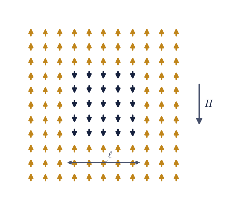
Fig. 505 The seeded-droplet geometry of the committor measurement, shown here on an \(11\times11\) patch with a \(5\times5\) seed. Up spins (amber, pointing up) fill the metastable phase and a centred square block of side \(\ell\) has been turned down (ink, pointing down) by hand to make a droplet of the stable phase; the applied field \(H\) points down, so the interior of the block is the favoured orientation and its boundary of length \(4\ell\) is what the droplet must pay for. Squares rather than discs are seeded because a square of side \(\ell\) has a perimeter of exactly \(4\ell\) on this lattice, whereas a rasterized disc has a ragged one, and Eq. 5 is the prediction for exactly this shape.#
critical droplet from seeded-droplet survival (T = 1.5, L = 36, 120 runs each):
  |H| = 0.15:  ell_50 =  9.67   CNT ell_c =  8.04 (square, eq-nuc-square)   ratio 1.20   ell_50*|H| = 1.450
  |H| = 0.20:  ell_50 =  7.59   CNT ell_c =  6.03 (square, eq-nuc-square)   ratio 1.26   ell_50*|H| = 1.517
  |H| = 0.25:  ell_50 =  6.44   CNT ell_c =  4.83 (square, eq-nuc-square)   ratio 1.33   ell_50*|H| = 1.610
  ell_50*|H| varies by 11.0% across the three fields (CNT: exactly constant at sigma/m_s = 1.206)
Validation 4#
✓ the measured critical droplet scales as 1/|H|, as classical nucleation theory requires when sigma/Delta f is the only length in the problem, and sits within 60% of the sharp-interface square-droplet prediction [ell_50*|H| spread = 11.0%, ratios to CNT = [1.2, 1.26, 1.33]]
True
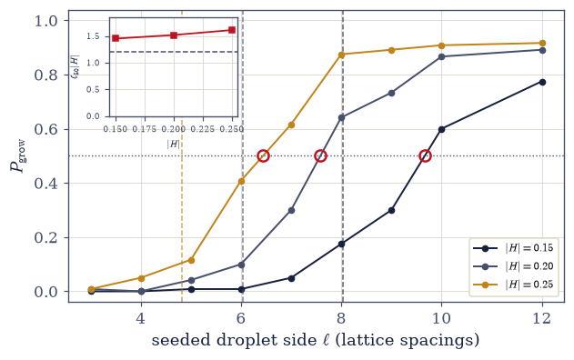
Fig. 506 Which seeded droplets survive. The probability that a square droplet of side \(\ell\), planted in a metastable \(36\times36\) Ising lattice at \(T=1.5\), grows to three times its area rather than vanishing, measured over 120 independent runs per point at three field strengths. The curves rise from zero to one across a window a few lattice spacings wide, and the dashed vertical lines mark the sharp-interface critical side \(\ell_c=2\sigma/\Delta f\) of Eq. 5 with Onsager’s \(\sigma\) and \(m_s\); the measured half-way crossings (circles on the grey line) sit consistently above it, since a seeded square is not the equilibrium droplet shape and carries excess perimeter it has to shed before it can grow. Inset: the crossings rescaled by the field, \(\ell_{50}|H|\), which classical nucleation theory says must be a constant.#
Exercise 5 — The critical droplet, route two: a free energy read off a histogram (worked)#
The committor found the saddle by watching the dynamics fall off it. The other route is thermodynamic and needs no dynamics at all, only the equilibrium statistics of the metastable phase. If \(n(s)\) is the number of clusters of size \(s\) per lattice site in the metastable basin, then those clusters are Boltzmann-distributed over their free energy of formation and
so a histogram of cluster sizes is a free-energy profile along the droplet-size coordinate, measured rather than modelled. The droplet picture predicts its shape: a perimeter term rising as \(\sqrt s\), because a compact cluster of area \(s\) has a boundary of length proportional to \(\sqrt s\), minus the bulk term \(\Delta f\,s\) of Eq. 479 that the field supplies.
Two things can be checked against exact answers, and they are worth checking first because they certify the histogram before anything is fitted to it. At \(H=0\) a single overturned spin has four unsatisfied bonds and no alternative shape, so its formation free energy is exactly \(8J\) with no entropy correction whatever the temperature. A two-site cluster has six unsatisfied bonds and exactly two orientations, horizontal or vertical, so its free energy is \(12J-kT\ln2\). Those are the first two points of the histogram, known in closed form.
The field term is then isolated in a way that owes nothing to droplet shapes at all. Run the same measurement twice, once at \(H=0\) and once at \(H\ne0\); the surface cost of a given cluster is the same in both, so the whole difference is the bulk term,
a straight line through the origin whose slope is Onsager’s \(2|H|m_s\) and nothing else. That is the sharpest quantitative statement in the notebook, and it is a genuine prediction: the slope was computed from the exact solution before any lattice was swept.
Where this route stops, and why. The histogram is a free energy only where there are counts, and a plain Metropolis run in the metastable basin produces clusters of size \(10\) perhaps once in a million site-samples and clusters of the critical size essentially never. That is not a defect of the measurement; it is the barrier, seen from the sampling side. Climbing it needs a method that biases the simulation towards the sizes it never visits and then removes the bias — umbrella sampling, or forward-flux sampling for the dynamical version — and this notebook deliberately does not use one. §5.11 hands rare-event and free-energy methods outward to molecular-simulation courses, and running at driving strong enough that nucleation happens unaided is how we honour that. So the barrier here is obtained by fitting the two terms where the statistics exist and extrapolating Eq. 481 to the saddle, which is exactly what classical nucleation theory does and exactly as trustworthy. The extrapolation is worth doing precisely because it shows its own weakness: the surface coefficient fitted to clusters of ten sites is not Onsager’s asymptotic \(4\sigma\) but something appreciably larger, because a cluster that small is mostly corners and has not yet acquired the wandering entropy that softens a long wall. It must lie between \(4\sigma\) and the entropy-free \(T=0\) perimeter cost \(8J\), and it does; but squaring it and dividing by \(\Delta f\) magnifies the gap, so the extrapolated barrier is substantially larger than the asymptotic one. Reaching the saddle honestly needs the sampling method we are not using, and this is what that costs.
Sampling is pooled over 60 independent preparations of a \(64\times64\) lattice, a snapshot every second sweep for at most 60 snapshots, and a run is abandoned the moment its magnetization drops below \(0.8\), since past that point the lattice is decaying rather than fluctuating.
cluster free energy F(s) = -kT ln n(s) at T = 1.5, L = 64 (3600 pooled snapshots at H = 0):
  F(1) = 8.032  vs exact 8J          (a single flipped spin, 4 broken bonds)
  F(2) = 11.060  vs exact 12J - kT ln2 = 10.960  (2 orientations)
  the field term, isolated as F_0(s) - F_H(s) over s = 1...10:
    |H| = 0.15:  slope 0.3029   predicted 2|H|m_s = 0.2959   ratio 1.023
    |H| = 0.25:  slope 0.4907   predicted 2|H|m_s = 0.4932   ratio 0.995
  surface term over the same range: F_0(s) ~ 6.16 sqrt(s), bracketed by Onsager's 4*sigma = 4.76 (asymptotic) and 8J (the T = 0 perimeter cost, no entropy yet)
  extrapolating those two fitted terms to the saddle, against CNT with Onsager's sigma:
    |H| = 0.15:  barrier  31.3 vs  19.1  (the fit overshoots by 64%, all of it from the surface coefficient)
    |H| = 0.25:  barrier  19.3 vs  11.5  (the fit overshoots by 68%, all of it from the surface coefficient)
  largest cluster with any counts at H = 0: s = 18   (the critical size is 23 sites at |H| = 0.25 and 65 at |H| = 0.15 — the sampling stops short)
Validation 5#
✓ the measured cluster free energy reproduces the exact one-spin cost 8J and the exact two-spin cost 12J - kT ln 2, the field term isolated between two histograms has Onsager's slope 2|H|m_s at both fields, and the surface coefficient of clusters this small lies between the asymptotic 4 sigma and the entropy-free T = 0 perimeter cost 8J [F(1) off by 0.40%, F(2) by 0.91%, bulk slopes / 2|H|m_s = [1.023, 0.995], surface coefficient 6.16 in (4.76, 8)]
True
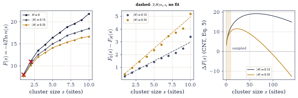
Fig. 507 The droplet free energy, measured and extrapolated. Left: \(F(s)=-kT\ln n(s)\) from pooled cluster-size histograms of a \(64\times64\) metastable lattice at \(T=1.5\), at \(H=0\) (ink) and at \(|H|=0.15\) and \(0.25\) (greys and amber); the two exact anchors \(F(1)=8J\) and \(F(2)=12J-kT\ln2\) are marked with red crosses, and the curves simply stop where the sampling runs out of counts at \(s\approx12\). Centre: the difference \(F_0(s)-F_H(s)\), which the droplet picture says is the pure bulk term \(2|H|m_s\,s\) with no shape dependence at all, against that prediction (dashed) computed from Onsager’s exact magnetization. Right: the classical-nucleation-theory profile \(4\sigma\sqrt{s}-\Delta f\,s\) of Eq. 5 drawn out to the saddle, with the sampled window shaded; the barrier top sits two decades of probability beyond anything an unbiased run visits, which is what umbrella sampling exists to reach and what this notebook declines to do.#
Exercise 6 — Which regime are we actually in? (student)#
Every picture so far has assumed the textbook story: one critical droplet appears somewhere, and grows until it has taken the lattice. That story is a regime, not a fact, and it is worth finding out whether the parameters everyone uses are inside it. Rikvold, Tomita, Miyashita and Sides [RTMS94] divide the metastable lifetime of exactly this model into four field regimes, and only one of them is the single-droplet picture. The competition is between the waiting time \(\tau\) for a droplet to appear anywhere and the time \(L/v\) for a droplet to sweep the lattice at its growth velocity. Because the nucleation rate is proportional to the number of sites, doubling \(L\) makes the wait four times shorter but the crossing only twice as long, so increasing the system size drives it out of the single-droplet regime, and it does so at a field that shrinks only as \(1/\ln L\). There is no comfortable lattice size.
Both regimes leave fingerprints that the lifetimes of Exercise 2 already contain, and neither needs anything new to be built.
In the single-droplet regime the decay is one memoryless event whose probability per sweep is proportional to the number of sites, so \(\tau\propto L^{-2}\) and the product \(\tau L^{2}\) is independent of \(L\), while the lifetime is exponentially distributed and its standard deviation equals its mean. In the multi-droplet regime many droplets nucleate independently and the lattice fills by their coalescence, so the decay time is an average over many events: it becomes nearly deterministic, its relative width falls well below one, and it stops shrinking as \(L^{-2}\) because the growth of the droplets rather than the wait for one now sets the clock. The two diagnostics are the constancy of \(\tau L^{2}\) and the ratio of standard deviation to mean, and a single sweep over lattice sizes at fixed field measures both.
We run at \(|H|=0.30\), and include \(L=40\) deliberately: that is the lattice of Exercise 11.4 of [Set21], at the same temperature and very nearly the same field.
Part a) Using the lifetime of Exercise 2, collect 60 lifetimes at \(T=1.5\), \(|H|=0.30\) for
each of \(L=12,16,24,32,40,48,64\) from seeds \(900\ldots959\) with max_sweeps=60000, and report
\(\tau\), \(\tau L^{2}\) and the ratio of standard deviation to mean for each.
Part b) Identify the plateau of \(\tau L^{2}\) over the three smallest lattices and report how far the largest lattice has departed from it, and where \(L=40\) falls.
Part c) Plot \(\tau L^{2}\) and the relative width against \(L\) on the same figure, marking the single-droplet expectations (a horizontal line, and unity) and the position of the textbook lattice.
metastable lifetime across lattice size at T = 1.5, |H| = 0.3 (60 runs each):
     L      tau      tau*L^2    tau*L^2 / plateau    std/mean
    12     605.7       87223        0.97            1.21
    16     352.6       90274        1.00            1.01
    24     160.4       92390        1.03            0.82
    32     119.3      122197        1.36            0.71
    40      96.3      154133        1.71            0.61   <- Sethna's 40x40
    48      79.7      183590        2.04            0.44
    64      66.1      270609        3.01            0.25
  single-droplet plateau over L = 12, 16, 24: 89963 (flat to 3.0%), with std/mean near 1 — one memoryless event
  by L = 64 the product has risen 3.0x and the width has fallen to 0.25 — many droplets, averaging into a near-deterministic filling
Validation 6#
✓ the single-droplet regime is identified by two independent fingerprints and both fail together at large L: tau*L^2 is flat and the lifetime width is 1 for L <= 24, while at L = 64 the product has more than doubled and the distribution has narrowed — the crossover Rikvold et al. describe [plateau flat to 3.0%, std/mean 1.01 -> 0.25, tau*L^2 up 3.0x]
True
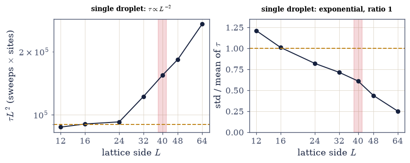
Fig. 508 Where the single-droplet picture stops being true. Both quantities are measured from 60 seeded metastable decays of a square Ising lattice at \(T=1.5\) and \(|H|=0.30\). Left: the product \(\tau L^{2}\) of the mean lifetime and the number of sites, which is constant (dashed, fitted on the three smallest lattices) exactly while decay is one rare event whose probability is proportional to the number of available sites, and which climbs once several droplets nucleate before any one of them can cross the lattice. Right: the ratio of the lifetime’s standard deviation to its mean, which is \(1\) (dashed) for the exponential distribution of a single memoryless event and falls towards zero as the decay becomes an average over many. The red band marks the \(40\times40\) lattice used in the standard textbook exercise at these very parameters; by both diagnostics it lies past the crossover, so the clean one-droplet story it tells is not the one the simulation is running.#
Exercise 7 — The lifetime against the field, and Onsager’s coefficient (student)#
The barrier of Eq. 480 scales as \(1/|H|\), so the Arrhenius law Eq. 483 predicts something unusually specific: not that the lifetime grows as the driving weakens, which is obvious, but that the logarithm of the lifetime is linear in the inverse field, with a slope fixed entirely by Onsager’s exact numbers, \(\Xi=\pi\sigma^{2}/(2m_skT)=1.503\) for the circular convention and \(2\sigma^{2}/(m_skT)=1.914\) for the square one. Measuring \(\ln\tau\) over a range of fields and reading off the slope is therefore a test with no adjustable parameters in it at all.
The measurement runs at \(L=24\), which Exercise 6 placed squarely on the single-droplet plateau at \(|H|=0.30\), and over the five fields \(|H|=0.22,0.25,0.28,0.31,0.34\). That window is narrow, and it is narrow for a reason worth stating: weaker fields make the lifetime grow exponentially past what a notebook can afford, while stronger fields shrink the critical droplet towards a single lattice spacing, where a sharp-interface theory has nothing left to describe. Roughly a factor of thirty in the lifetime is what fits between those two walls.
A straight line through five points is easy to obtain and easy to over-read, so the fit is judged against a rival rather than against itself. If the lifetime were governed by a power law \(\tau\propto|H|^{-n}\) instead of by a barrier, \(\ln\tau\) would be linear in \(\ln|H|\) rather than in \(1/|H|\); fitting both and comparing the coefficients of determination asks the data which functional form it prefers, which is a question it can answer and a question it can answer the other way.
One honest caveat travels with the slope. What Eq. 483 calls a constant prefactor is not constant: the Becker–Döring theory this notebook declines to develop gives it its own power of \(|H|\), which adds to the apparent slope over a narrow window. So a measured slope somewhat above \(\Xi\) is expected, and separating the two contributions would need a field range we cannot reach.
Part a) Using the lifetime of Exercise 2, collect 48 lifetimes at \(T=1.5\), \(L=24\) for each
of \(|H|=0.22,0.25,0.28,0.31,0.34\) from seeds \(500\ldots547\) with max_sweeps=40000.
Part b) Fit \(\ln\tau\) against \(1/|H|\) with numpy.polyfit of degree 1, and separately fit
\(\ln\tau\) against \(\ln|H|\); report both coefficients of determination and both slopes.
Part c) Compare the fitted barrier coefficient with \(\Xi\) from Eq. 483 in both the circular and the square convention, and plot \(\ln\tau\) against \(1/|H|\) with the fitted line and the two theoretical slopes drawn through the data.
metastable lifetime against field at T = 1.5, L = 24 (48 runs per field):
  |H| = 0.22   1/|H| =  4.55   tau =   2009.0   ln tau =  7.61
  |H| = 0.25   1/|H| =  4.00   tau =    645.3   ln tau =  6.47
  |H| = 0.28   1/|H| =  3.57   tau =    251.7   ln tau =  5.53
  |H| = 0.31   1/|H| =  3.23   tau =    119.4   ln tau =  4.78
  |H| = 0.34   1/|H| =  2.94   tau =     78.0   ln tau =  4.36
  Arrhenius fit  ln tau = 2.064/|H| + -1.800     R^2 = 0.9977
  power-law fit  ln tau = -7.59 ln|H| + const          R^2 = 0.9894
  the barrier coefficient Xi of eq-nuc-arrhenius, from Onsager alone:
    circular droplet  1.503   (measured / predicted = 1.37)
    square droplet    1.914   (measured / predicted = 1.08)
  lifetime spans a factor of 26 across the window
Validation 7#
✓ ln(lifetime) is linear in 1/|H| rather than in ln|H| — a barrier, not a power law — and its slope matches the square-droplet coefficient 2 sigma^2/(m_s kT) built from Onsager's exact tension and magnetization, with no fitted input [R^2 = 0.9977 (power law 0.9894), slope 2.064 vs Xi_square = 1.914, Xi_circle = 1.503]
True
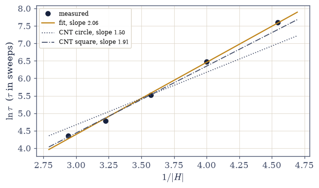
Fig. 509 The Arrhenius law of nucleation, with no fitted physics in the prediction. Mean metastable lifetimes of a \(24\times24\) Ising lattice at \(T=1.5\), 48 seeded runs per field, plotted as \(\ln\tau\) against the inverse field \(1/|H|\), the variable in which Eq. 7 says the barrier makes the relation straight. The amber line is the least-squares fit; the two dotted lines carry the slopes \(\Xi=\pi\sigma^{2}/(2m_skT)\) and \(2\sigma^{2}/(m_skT)\) predicted for a circular and a square critical droplet from Onsager’s exact interfacial tension and spontaneous magnetization, drawn through the central datum so only their gradients are being compared. The measurement sits just above the square-droplet slope, as it should: the rate prefactor this notebook does not compute carries its own field dependence, which adds to the apparent gradient over a window this narrow.#
Exercise 8 — Nucleation is not coarsening (worked)#
§5.10 already animated a lattice that starts disordered and ends up magnetized, and it looks superficially like the animation of Exercise 3. The two processes are different in kind, and confusing them is a standing hazard because both are done on the same model with the same sampler. Sethna keeps them as separate exercises for exactly this reason [Set21], and so should we.
In a temperature quench the system is cooled from above \(T_c\) to below it at zero field. The state it arrives in, \(m=0\), is not metastable but unstable: there is no barrier at all, ordered domains begin growing from the first sweep, and what follows is coarsening, the slow elimination of domain walls as small domains are swallowed by large ones. The driving force is surface tension alone, the field plays no part, and because the \(\mathbb{Z}_2\) symmetry of Eq. 477 is untouched at \(H=0\), which sign finally wins is decided by chance. The characteristic domain size grows as a power of time, so the excess energy carried by the walls falls as a power of time from the very first sweep.
In a field reversal at fixed temperature, which is this notebook’s experiment, the state the system finds itself in is metastable rather than unstable, the field breaks the symmetry outright, and the outcome is never in doubt: the lattice will end up aligned with the field. What is in doubt is when, and the waiting is the whole phenomenon.
Two measurements separate them cleanly, and both are checks that could come out the other way. The first is the outcome: over 40 quenches the final sign should be a coin flip, while over 40 field reversals it should be the field’s sign every single time. The second is the kinetics: after a quench the excess bond energy \(\varepsilon(t)-\varepsilon_{\rm eq}\) should decay as a power law immediately, with no waiting time at all, while after a field reversal it should sit flat until nucleation happens. We measure the coarsening exponent as well, without claiming more than the data supports: the asymptotic Allen–Cahn value for a non-conserved order parameter is \(1/2\), and the effective exponent at the early times a notebook can afford is measurably steeper, because the domains are still only a few interface widths across.
Part a) Run 40 temperature quenches from a random configuration to \(T=1.5\) at \(H=0\) on a \(32\times32\) lattice for 400 sweeps, and count how many end with \(m>0\).
Part b) Run 40 field reversals at \(T=1.5\), \(|H|=0.25\) on the same lattice with the
metastable_run of Exercise 2, stopping each at \(m<-0.5\) or 1500 sweeps, and count how many end
negative.
Part c) Measure the equilibrium bond energy per site of the ordered phase at \(T=1.5\), then
average the excess bond energy over 12 quenches of a \(96\times96\) lattice for 250 sweeps and fit
\(\ln(\varepsilon-\varepsilon_{\rm eq})\) against \(\ln t\) over \(t\in[10,200]\) with
numpy.polyfit, reporting the exponent and its coefficient of determination.
coarsening (quench in temperature) against nucleation (reversal of the field):
  quench, H = 0:      20/40 runs end with m > 0 — the Z2 symmetry is intact and the sign is a coin flip
  field reversal:     40/40 runs end aligned with the field — the outcome was never in doubt, only its timing
  equilibrium bond energy per site at T = 1.5: -1.9502
  excess bond energy after a quench decays as t^(-0.71) over t in [10, 200], R^2 = 0.9863
  (the asymptotic Allen-Cahn exponent is -1/2; at these early times the measured decay is steeper, since the domains are still only a few walls wide)
Validation 8#
✓ a temperature quench and a field reversal are different processes: the quench keeps the Z2 symmetry and picks its sign at random while every reversal ends aligned with the field, and the quench's wall energy decays as a power law from the first sweep instead of waiting behind a barrier [quench 20/40 positive, reversal 40/40 negative, coarsening exponent -0.71 (R^2 = 0.986)]
True
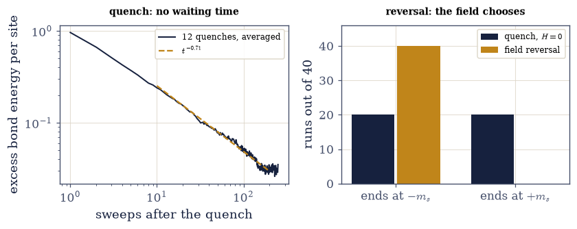
Fig. 510 Two ways to make an Ising lattice order, and they are not the same physics. Left: the excess nearest-neighbour bond energy above its equilibrium value, which measures how much domain wall a configuration still carries, averaged over 12 quenches of a \(96\times96\) lattice from a random configuration to \(T=1.5\) at zero field; on logarithmic axes it is a straight line from the first sweep, the signature of coarsening driven by surface tension with no barrier to wait behind, and the amber line is the fitted power law. Right: the distribution of final magnetizations over 40 runs of each kind at \(T=1.5\); the quench (ink) splits evenly between \(+m_s\) and \(-m_s\) because at \(H=0\) nothing distinguishes them, whereas every field reversal (amber) ends at \(-m_s\), since the field decided the outcome at the start and left only the timing to chance.#
With your assistant
Ask your assistant for a different reaction coordinate for the critical droplet — the largest cluster in the whole lattice rather than the one containing the centre, or the total minority area, or the perimeter instead of the area — and rebuild the committor of Exercise 4 on it. The gate is the scaling law, not the number: whatever coordinate it proposes, the half-way crossing must still fall as \(1/|H|\) across \(|H|=0.15\), \(0.20\) and \(0.25\) to the same 15% this notebook measured, and any coordinate for which it does not is telling you it is not tracking the droplet. The check is yours.
Notebook summary#
We gave the Ising model of §5.10 an external field, which cost two lines of code and bought a genuinely new phenomenon: a phase that is wrong and stable at the same time.
The field in the energy Eq. 477, Eq. 478: \(\Delta E_i=2\sigma_i(\sum_j\sigma_j+H)\), with the field inside the bracket. Certified against a brute-force energy difference at every site (agreement to \(9\times10^{-16}\)), against the zero-field sweep of §5.10 bitwise at \(H=0\) on a configuration in which half the sites move, and against itself at \(H=0.4\), where the two sweeps part company at 86% of sites.
Metastability is a waiting time, not a drift. After reversing the field at \(T=1.5\), \(|H|=0.25\), the magnetization holds at \(+m_s=0.9865\) and then collapses. Over 150 seeded runs at \(L=24\) the lifetime came out exponentially distributed, with standard deviation \(0.88\) of the mean and a survival curve straight on a logarithmic axis to \(R^{2}=0.99\): the decay is one memoryless rare event.
The critical droplet, measured twice. Seeding squares and asking which survive gave \(\ell_{50}=9.7\), \(7.6\) and \(6.4\) at \(|H|=0.15\), \(0.20\), \(0.25\), so \(\ell_{50}|H|\) is constant to \(11\%\) — the \(1/|H|\) scaling Eq. 481 demands — sitting \(20\) to \(33\%\) above the sharp-interface prediction, since a seeded square carries perimeter the equilibrium shape does not.
The free energy, read off a histogram Eq. 485. Cluster statistics reproduced the exact costs \(F(1)=8J\) (measured \(8.03\)) and \(F(2)=12J-kT\ln2\) (measured \(11.06\) against \(10.96\)), and the difference between the \(H=0\) and \(H\neq0\) histograms isolated the bulk term with slope \(0.303\) and \(0.491\) against Onsager’s \(2|H|m_s=0.296\) and \(0.493\). The surface coefficient of ten-site clusters came out \(6.16\), between the asymptotic \(4\sigma=4.76\) and the entropy-free \(8J\), which is why extrapolating this route to the barrier overshoots by two thirds.
The Arrhenius law Eq. 483: \(\ln\tau=2.064/|H|-1.80\) across a factor of \(26\) in lifetime, with \(R^{2}=0.998\) against \(0.989\) for the power-law rival, and the slope within \(8\%\) of the square-droplet coefficient \(2\sigma^{2}/(m_skT)=1.914\) assembled from Onsager’s exact tension and magnetization with nothing fitted.
The regime, checked rather than assumed. \(\tau L^{2}\) is flat to \(3\%\) and the lifetime width is \(1\) for \(L\le24\), and by \(L=64\) the product has tripled and the width has fallen to \(0.25\). The \(40\times40\) lattice of the standard textbook exercise, at the same temperature and very nearly the same field, sits at \(1.7\) times the plateau with a width of \(0.61\): past the crossover Rikvold and co-workers describe [RTMS94], and therefore not running the one-droplet story it is used to illustrate.
Coarsening is a different process. A temperature quench ends at \(+m_s\) in \(20\) of \(40\) runs and loses wall energy as a power law from the first sweep; a field reversal ends aligned with the field in \(40\) of \(40\) and does nothing at all until it nucleates.
What we did not compute, and said so at every opportunity: the rate prefactor, which is Becker–Döring kinetics and a Fokker–Planck equation in cluster-size space, and which is also the reason the fitted slope \(2.064\) sits a little above the barrier coefficient it is compared with.
Outlook#
The prefactor, and the kinetics behind it. Everything here lives in the exponent. The rate in front of it needs the probability current through the saddle in cluster-size space: the Becker–Döring master equation, its continuum Fokker–Planck limit, and Zeldovich’s factor for the fraction of critical droplets that recross rather than commit. Landau and Lifshitz, Physical Kinetics §99 [LP81] develops it in full, importing the barrier from equilibrium statistical mechanics exactly as we did. Kramers’ escape problem is the same mathematics in one dimension.
Reaching the barrier top honestly. Exercise 5 stopped where the counts ran out, which is two decades of probability short of the saddle. Umbrella sampling biases the simulation towards the cluster sizes it never visits and removes the bias afterwards; forward-flux and transition interface sampling do the dynamical version, and give the rate rather than only the free energy. These belong to the molecular-simulation courses §5.11 points to, and to the Materials Modelling course.
Heterogeneous nucleation, which is what actually happens. Real systems almost never nucleate in the bulk: a wall, a dust grain, or a scratch on a mug offers a surface that removes part of the droplet’s perimeter and therefore part of the barrier. A single fixed down spin held in this lattice would show it immediately, and it is why a boiling chip works and why superheated water in a smooth mug does not.
The same barrier, everywhere else. The competition between a perimeter and an area is not about magnets. It is the condensation of a droplet in a cloud chamber, the birth of a bubble in a superheated liquid, the precipitation of a second phase in an alloy, the folding nucleus of a protein, and the metastable strip of §5.15 between binodal and spinodal that sent us here. Change what \(\sigma\) and \(\Delta f\) mean and the arithmetic is untouched.
Cross-reference §5.10 (the model, the sampler, and the sibling temperature quench), §5.8 (Metropolis), §5.15 (the metastable strip), §5.17 (blocked error bars on correlated Monte Carlo output), and E.3 (measuring a scaling claim rather than asserting it).
References#
Harvey Gould, Jan Tobochnik, and Wolfgang Christian. An Introduction to Computer Simulation Methods: Applications to Physical Systems. Addison-Wesley, San Francisco, 3 edition, 2007.
E. M. Lifshitz and L. P. Pitaevskii. Physical Kinetics. Volume 10 of Course of Theoretical Physics. Pergamon Press, Oxford, 1981.
Per Arne Rikvold, H. Tomita, S. Miyashita, and Scott W. Sides. Metastable lifetimes in a kinetic ising model: dependence on field and system size. Physical Review E, 49:5080–5090, 1994. doi:10.1103/PhysRevE.49.5080.