


5.3 The Large-N Limit: Stirling, the CLT, and Sharp Macrostates#
Notebook overview#
This is the last notebook of Volume V’s mathematical arsenal, and the one where the arsenal turns into physics. Counting (§5.1) and probability (§5.2) gave us the tools; here we take them to the limit that statistical mechanics actually lives in, \(N\sim10^{23}\), and three things happen that together make thermodynamics possible.
First, a computational wall. The factorials that count microstates grow so fast that
\(1000!\) overflows a 64-bit float outright — a direct return of the floating-point limits of
§0.1. The escape is to stop computing the count and compute its logarithm, with
scipy.special.gammaln, and this is not a mere trick: statistical mechanics is written in log
space because that is the only space its numbers fit in. Stirling’s approximation then
turns \(\ln N!\) into a clean closed form, the analytic handle that converts a factorial count
into an entropy.
Second, a universal law. The central limit theorem says that the sum of many independent random variables, whatever their individual distribution, approaches a Gaussian. We watch a perfectly flat distribution become a bell curve in about thirty steps, and we see the binomial of a two-state system do the same. The Gaussian is not one distribution among many; it is the large-\(N\) attractor of nearly all of them.
Third, and deepest, sharpness. For \(N\) independent contributions the sum has mean proportional to \(N\) but standard deviation only proportional to \(\sqrt N\), so the relative fluctuation falls as \(1/\sqrt N\). At Avogadro’s number that is about one part in \(10^{12}\): the spread is so negligible that a thermodynamic variable — an energy, a pressure, a temperature — has an effectively exact value. Macroscopic determinism, the whole edifice of thermodynamics, is the law of large numbers in disguise. We close by assembling these pieces into the entropy of mixing, \(S=k\ln\Omega\), the first formula of statistical mechanics and the hand-off to the physics that begins at §5.4.
We reuse the distribution-bar plots and Monte Carlo machinery of §5.1–§5.2, verify our
hand-built results against scipy where useful, and keep every \(N\) and distribution stated
explicitly.
How to read the checks. Each exercise closes with a
validatecall against an independent fact: factorials overflowing whilegammalnstays finite; Stirling matching \(\ln N!\); the sample mean converging; a sum of uniforms with mean \(N/2\) and standard deviation \(\sqrt{N/12}\) going Gaussian; the binomial→Gaussian limit; \(\sigma/\mu\propto1/ \sqrt N\); the mixing entropy approaching \(-\sum x_i\ln x_i\). A ✓ is strong evidence; a ✗ is a prompt to locate the discrepancy, not a verdict.Scope. The large-\(N\) limit that bridges the math arsenal to the physics; the physics proper — microstates, the Boltzmann distribution, temperature — begins at §5.4. See Schroeder, Thermal Physics; Kardar, Statistical Physics of Particles; Feller; and §0.1 (floating point), §5.1 (counting), §5.2 (probability).
Theory in brief#
The computational wall: factorials overflow#
A microstate count is a factorial, and factorials grow faster than any exponential. \(1000!\) has \(2568\) digits and overflows a \(64\)-bit float (\(\max\approx1.8\times10^{308}\)),
The remedy, a direct callback to §0.1, is to work with \(\ln N!\) throughout: statistical mechanics lives in log space.
Stirling’s approximation#
The logarithm has a beautifully simple large-\(N\) form,
The leading form is already good to \(\sim0.9\%\) at \(N=100\); the corrected one to \(\sim2\times 10^{-4}\%\). Stirling is the analytic handle that turns a factorial count into a closed-form expression, and the gateway to entropy. We verify the approximation numerically rather than derive it; Reif, Fundamentals of Statistical and Thermal Physics, App. A.6, carries the derivation out in full.
The law of large numbers and the central limit theorem#
Two limit theorems govern sums of \(N\) independent, identically distributed variables. The law of large numbers says the sample mean converges to the true mean,
and the central limit theorem says the fluctuations around it are Gaussian, whatever the distribution of each \(X_i\),
The Gaussian is the universal large-\(N\) attractor; the binomial→Gaussian case is the discrete instance (de Moivre–Laplace). We watch both theorems act rather than prove them; Feller, An Introduction to Probability Theory, supplies the proofs in full.
Fluctuations and the sharpness of macrostates#
Because the sum has mean \(\propto N\) and standard deviation \(\propto\sqrt N\), the relative fluctuation shrinks,
At macroscopic \(N\) the relative spread is utterly negligible, so a thermodynamic variable has an effectively sharp value. This is why thermodynamics is deterministic though built on chance.
The bridge to physics: entropy#
Stirling turns the log of a multiplicity into an extensive quantity. For \(N\) particles split into species with fractions \(x_i\),
This is the entropy of mixing, and \(S=k\ln\Omega\) is the first formula of statistical mechanics: entropy is the logarithm of a count, computable only in log space, extensive and sharp only because \(N\) is large.
Setup#
Data only, plus the series palette and Avogadro’s number. Nothing this notebook is about
is here: the two Stirling forms Eq. 393 you write in Exercise 2, the log-space
multiplicity log_multiplicity in Exercise 7, and the log-binomial log_binomial in
Exercise 8. Those are the objects the lesson is named for, and the reference they are all
graded against, scipy.special.gammaln, is a library call. Each exercise that needs
randomness seeds its own generator in view, so no rng lives here either.
The Setup below holds this notebook’s data and instruments — nothing you are asked to build. It is collapsed so the building stays yours; expand it whenever you want the details.
Exercise 1 — The factorial wall and log space (worked)#
Statistical mechanics counts microstates, and microstate counts are factorials, and factorials
are where ordinary arithmetic breaks. We met the limits of floating point in §0.1; here
they bite hard. The number \(1000!\) has \(2568\) digits, far past the \(\sim308\)-digit ceiling of a
\(64\)-bit float, so asking for it as a float overflows to infinity. The escape is to never
compute the count itself but its logarithm, \(\ln N!=\ln\Gamma(N+1)\), which
scipy.special.gammaln evaluates directly and without overflow Eq. 392. From here
on we live in log space, because the numbers of statistical mechanics simply do not fit
anywhere else. Every entropy in this volume is a gammaln, never a factorial.
Part a) Show that converting \(1000!\) to a float overflows, by catching the
OverflowError that float(math.factorial(1000)) raises, and that
scipy.special.gammaln(1001) returns a finite \(\ln(1000!)\) instead.
Part b) Confirm that gammaln(n+1) really is \(\ln n!\), by comparing it against
math.log(math.factorial(n)) for \(n=1,\dots,10\) (the range where the exact factorial is
still small enough to form).
Part c) Tabulate \(\ln N!\) for \(N=10,\,10^2,\,10^3,\,10^6\) and \(10^{23}\), sizes at which the factorial itself could never be written down at all.
float(1000!) overflows a 64-bit float: True
gammaln(1001) = ln(1000!) = 5912.128  (finite)
check gammaln(6) = 4.787492  vs  ln(5!) = 4.787492

   N        ln(N!)
  10       1.5104e+01
  100      3.6374e+02
  1000     5.9121e+03
  1000000   1.2816e+07
  100000000000000000000000   5.1959e+24
Validation 1#
✓  factorials overflow a float; their logarithms via gammaln do not
✓  gammaln(n+1) computes ln(n!)   [max|Δ| = 0 (rtol=1e-09, atol=1e-09)]
True
Exercise 2 — Stirling’s approximation (worked)#
Working in log space proves its worth immediately, because \(\ln N!\) has a remarkably simple large-\(N\)
form. Stirling’s approximation is \(\ln N!\approx N\ln N-N\), with a first correction
\(+\tfrac12\ln(2\pi N)\) Eq. 393. The leading form already tracks the exact value to
under a percent at \(N=100\), and the corrected form to a few parts in a million
(Fig. 406). This is the analytic lever of the whole subject: it replaces an
intractable factorial with elementary functions of \(N\), and it is what lets a log-multiplicity
collapse into a closed-form entropy in Exercise 7. The reference both forms are graded
against is scipy.special.gammaln, which evaluates \(\ln\Gamma\) to machine precision without
ever forming a factorial, so every discrepancy measured below is pure approximation error and
nothing else. Treat \(n\) as continuous throughout, so that both forms accept a whole numpy
array of sizes at once.
Part a) Write the two approximations of Eq. 393 as stirling_leading(n) and
stirling_corrected(n): the leading form \(n\ln n-n\), and the same expression with the first
correction \(+\tfrac12\ln(2\pi n)\) added.
Part b) Tabulate the relative error of both forms against the exact \(\ln N!\) for \(N=10,30,100,300,1000,3000,10000\), and plot the two error curves against \(N\) on log–log axes.
Part c) Confirm that the corrected form matches \(\ln N!\) to better than \(10^{-4}\) relative at \(N=1000\), and that both relative errors shrink as \(N\) grows.
    N     leading rel err    corrected rel err
  10       1.376e-01        5.515e-04
  30       3.512e-02        3.721e-05
  100      8.859e-03        2.291e-06
  300      2.665e-03        1.963e-07
  1000     7.396e-04        1.410e-08
  3000     2.341e-04        1.321e-09
  10000    6.728e-05        1.015e-10
Validation 2#
✓  Stirling's approximation (with the ½ln(2πN) term) matches ln(N!) at large N   [got 5912.13 vs expected 5912.13 (rtol=0.0001, atol=1e-09)]
✓  both Stirling relative errors shrink with N
True
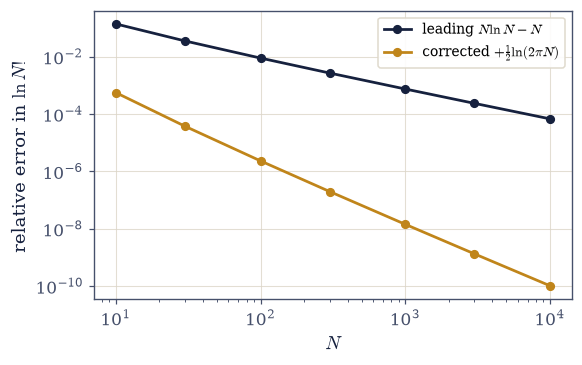
Fig. 406 Relative error of Stirling’s approximation to \(\ln N!\) against \(N\) (log–log). The leading form \(N\ln N-N\) (dark) is good to \(\sim0.9\%\) at \(N=100\) and falls as \(1/N\); the corrected form \(N\ln N-N+\tfrac12\ln(2\pi N)\) (amber) is already accurate to a few parts in \(10^{6}\) and falls faster still. By the \(N\) of statistical mechanics, Stirling is effectively exact — which is what lets a factorial count become a closed-form entropy.#
Exercise 3 — The law of large numbers (worked)#
Before the subtler limit theorem, the simple one. The law of large numbers says that the average of many independent draws converges to the true mean Eq. 394. Roll a fair die repeatedly and keep a running average: it wanders at first, then settles inexorably onto \(3.5\) (Fig. 407). This is the same convergence that made Monte Carlo work in §5.2, now named, and it is the first reason large systems behave predictably: averaged over enough constituents, chance washes out. A fair die has true mean \(3.5\) and standard deviation \(\sigma=\sqrt{35/12}\), so the spread of the running mean after \(N\) rolls is \(\sigma/\sqrt N\): that is the shrinking envelope drawn around the trace in the figure.
Part a) Draw \(100{,}000\) fair-die rolls with numpy.random.default_rng and form the
running sample mean with numpy.cumsum, then plot it against the number of rolls on a
logarithmic axis inside the \(3.5\pm\sigma/\sqrt N\) band.
Part b) Confirm that the running mean has converged to the true mean \(3.5\) by the end of the sequence.
true mean of a fair die = 3.5
sample mean after 100,000 rolls = 3.4984
Validation 3#
✓ the sample mean converges to the true mean (law of large numbers) [got 3.49844 vs expected 3.5 (rtol=0.01, atol=1e-09)]
True
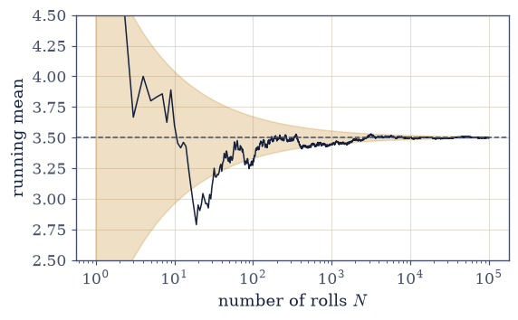
Fig. 407 The law of large numbers: the running mean of fair-die rolls (dark) converges to the true mean \(3.5\) (dashed) as the number of rolls grows. The amber envelope is the \(3.5\pm\sigma/\sqrt N\) band, the \(1/\sqrt N\) shrinking of the fluctuation about the mean — the same convergence that makes Monte Carlo estimates sharpen, and the first reason large systems are predictable.#
Exercise 4 — The central limit theorem from a flat distribution (worked)#
Here is the striking one. The central limit theorem says the sum of many independent variables tends to a Gaussian no matter what distribution each one has Eq. 395. To see how universal that is, start from the least Gaussian distribution imaginable: the flat uniform\([0,1]\). The sum of one is flat; the sum of two is a triangle; and by about thirty the sum is a bell curve indistinguishable from a Gaussian by eye (Fig. 408). The sum of \(N\) uniforms has mean \(N/2\) and variance \(N/12\), and its skewness and excess kurtosis (the third- and fourth-moment fingerprints of non-Gaussianity, both exactly zero for a Gaussian itself) march to zero. The animation morphs the standardized distribution from flat toward the Gaussian as \(N\) climbs.
Part a) With numpy.random.default_rng, draw \(200{,}000\) sums of \(N=30\) uniform\([0,1]\)
variables and confirm with numpy.mean and numpy.std that the sample mean and standard
deviation match \(N/2\) and \(\sqrt{N/12}\).
Part b) Tabulate the skewness and excess kurtosis of the sum for \(N=1,2,5,30\)
(scipy.stats.skew and scipy.stats.kurtosis, used for checking only) and confirm that both
fall toward zero as \(N\) grows, the flat base distribution leaving no trace.
sum of N=30 uniforms:
  mean = 15.0018  vs N/2     = 15.0
  std  = 1.5775  vs √(N/12) = 1.5811
    N     skewness    excess kurtosis
  1      +0.0042    -1.2030
  2      +0.0038    -0.5760
  5      -0.0026    -0.2417
  30     -0.0201    -0.0306
Validation 4#
✓  the sum of N uniforms has mean N/2 and standard deviation √(N/12)   [max|Δ| = 0.00360333 (rtol=0.01, atol=1e-09)]
✓  the sum approaches a Gaussian (excess kurtosis → 0) regardless of the flat base distribution
True
Fig. 408 The central limit theorem in action (animated). Each frame standardizes the sum of \(N\) uniform\([0,1]\) variables to zero mean and unit variance and histograms it; as \(N\) grows from \(1\) the distribution morphs from flat, through the triangle at \(N=2\), to a bell curve sitting on the standard Gaussian (dark) by \(N\approx30\). The flat base distribution is gone without trace — the Gaussian is the universal large-\(N\) attractor, which is why measurement errors and thermal fluctuations are Gaussian almost regardless of their microscopic origin.#
Exercise 5 — The binomial becomes Gaussian: de Moivre–Laplace (worked)#
The two-state system of §5.1 and §5.2 — coins, spins, the paramagnet — gives the discrete instance of the same limit. The de Moivre–Laplace theorem says the binomial\((N,\tfrac12)\) approaches a Gaussian of matching mean \(N/2\) and variance \(N/4\) as \(N\) grows Eq. 395. By \(N=100\) the two agree to a couple parts in \(10^4\) everywhere (Fig. 409). This is why the multiplicity of a large paramagnet — the number of ways to have \(k\) spins up — is a sharp Gaussian peak about \(k=N/2\), the fact we draw on for the sharpness of macrostates and, at §5.4, for its energy distribution. Nothing here is fitted: the comparison Gaussian takes the binomial’s own mean \(N/2\) and variance \(N/4\), so the two curves have no free parameter between them.
Part a) Build the exact binomial\((100,\tfrac12)\) probability mass function
\(\binom{N}{k}2^{-N}\) with math.comb (integer arithmetic, so the coefficients carry no
rounding), form the matched Gaussian on the same \(k\) axis, and plot the two together.
Part b) Confirm the maximum absolute difference between them is below \(10^{-3}\).
binomial(100, ½) vs matched Gaussian (mean 50.0, variance 25.0):
  maximum absolute difference = 1.99e-04
Validation 5#
✓ the binomial converges to a Gaussian (de Moivre–Laplace) [max|Δ| = 0.000199219 (rtol=1e-06, atol=0.001)]
True
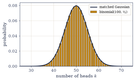
Fig. 409 The binomial\((100,\tfrac12)\) (amber bars) and the Gaussian of matching mean \(N/2=50\) and variance \(N/4=25\) (dark curve). They are indistinguishable to a couple parts in \(10^{4}\) — the discrete central limit theorem (de Moivre–Laplace). For a paramagnet of \(N\) spins this is the multiplicity: the number of ways to have \(k\) spins up is a sharp Gaussian about \(k=N/2\), the seed of the sharp macrostates of Exercise 8.#
Exercise 6 — Fluctuations shrink as 1/√N (worked)#
This is the payoff the whole arsenal was built for. Take \(N\) independent contributions to some extensive quantity. Their sum has mean proportional to \(N\) and, because variances add (§5.2), standard deviation proportional to \(\sqrt N\). The relative fluctuation is therefore the ratio, \(\sigma/\mu\propto1/\sqrt N\) Eq. 396, and it shrinks without bound as the system grows (Fig. 410). At \(N=100\) it is about \(10\%\); at \(N=10^4\), about \(1\%\); at Avogadro’s number it is about \(1.3\times10^{-12}\), one part in a trillion. That is the deepest fact in this notebook: at macroscopic \(N\) the relative spread of a thermodynamic variable is so small that the variable is, for all purposes, sharp. A mole of gas has a definite energy, pressure, and temperature not because chance has been banished but because the law of large numbers has made it invisible.
Part a) Tabulate the predicted relative fluctuation \(\sigma/\mu=1/\sqrt N\) for \(N=10^2,10^4,10^6,10^{12},10^{18}\) and Avogadro’s number, and confirm it reaches \(\approx1.3\times10^{-12}\) at a mole.
Part b) Verify the \(1/\sqrt N\) scaling directly rather than assuming it: with
numpy.random.default_rng, simulate \(20{,}000\) sums of \(N\) die rolls for
\(N=10,10^2,10^3,10^4\), measure \(\sigma/\mu\) with numpy.std and numpy.mean, and check that
\(\sigma/\mu\cdot\sqrt N\) is constant across the four sizes. Plot the measurements against the
\(1/\sqrt N\) line extrapolated out to Avogadro’s number.
       N            σ/μ (∝ 1/√N)
  1.00e+02      1.000e-01
  1.00e+04      1.000e-02
  1.00e+06      1.000e-03
  1.00e+12      1.000e-06
  1.00e+18      1.000e-09
  6.02e+23      1.289e-12
simulated σ/μ × √N (should be ~constant): [0.4867 0.4882 0.4869 0.4836]
Validation 6#
✓  the relative fluctuation scales as 1/√N   [max|Δ| = 0.00308044 (rtol=0.05, atol=1e-09)]
✓  at Avogadro's number the relative fluctuation is ~10⁻¹²   [got 1.28862e-12 vs expected 1.3e-12 (rtol=0.05, atol=1e-09)]
True
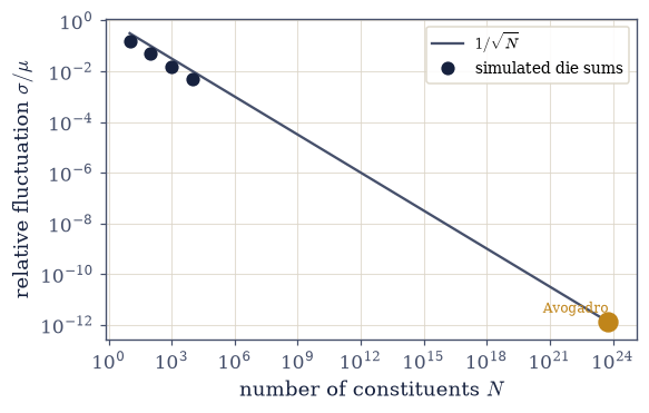
Fig. 410 The relative fluctuation \(\sigma/\mu=1/\sqrt N\) against system size (log–log), from a handful of particles to Avogadro’s number (amber dot, \(\sim1.3\times10^{-12}\)). Simulated sums of die rolls (dark dots) sit exactly on the \(1/\sqrt N\) line. This is why macroscopic determinism exists: at a mole the relative spread of energy or pressure is one part in a trillion, so a thermodynamic variable has an effectively exact value, and the laws built on it are deterministic.#
Exercise 7 — From a count to an entropy: the entropy of mixing (worked)#
Now the bridge, where the math arsenal becomes physics. The number of ways to arrange \(N\) particles of two species, \(N_A\) of one and \(N_B\) of the other, is the multiplicity \(\Omega= N!/(N_A!\,N_B!)\) — a single binomial coefficient, far too large to compute directly but perfectly tractable in log space Eq. 397. Feed \(\ln\Omega\) through Stirling and the factorials collapse into something extensive and physical,
the entropy of mixing per particle, with \(x_i=N_i/N\). Multiply by Boltzmann’s constant and this is \(S=k\ln\Omega\), the first formula of statistical mechanics. Everything we built points here: entropy is the logarithm of a count (§5.1), made finite by working in log space (this notebook, and §0.1), and extensive only because Stirling’s sub-leading terms vanish per particle as \(N\) grows (Fig. 411). For the mixture used below, \(x_A=0.3\) and \(x_B=0.7\), the limit is \(-\sum_i x_i\ln x_i=0.611\).
Part a) Write log_multiplicity(counts), the log-multiplicity
\(\ln\Omega=\ln\!\big(N!/\prod_i N_i!\big)\) of a mixture whose species counts are the entries
of counts Eq. 397. Never form \(\Omega\), and never form a factorial: with
\(N=\sum_i N_i\), split the logarithm into \(\ln N!-\sum_i\ln N_i!\) and evaluate every term as
scipy.special.gammaln\((\,\cdot+1)\), so the computation stays in log space and cannot
overflow at any \(N\). Write this one yourself — the implementation is the lesson: this
rewrite is the whole reason an entropy is computable at all, and it is the piece of machinery
the rest of the volume runs on.
Part b) For \(N=100,1000,10000\) at \(x_A=0.3\), compute \(\ln\Omega\) two independent ways
(exactly, with your log_multiplicity, and through the stirling_corrected you wrote in
Exercise 2, as stirling_corrected(N) - stirling_corrected(N_A) - stirling_corrected(N_B))
and confirm the two agree at the largest \(N\).
Part c) Show that the per-particle value \(\ln\Omega/N\) converges to \(-\sum_i x_i\ln x_i\) as \(N\) grows: the sub-leading Stirling terms, which scale as \(\ln N/N\), vanish per particle, which is what leaves the entropy extensive.
mixing fractions x_A=0.3, x_B=0.7;  −Σ xᵢ ln xᵢ = 0.61086
     N      lnΩ (gammaln)     lnΩ (Stirling)    per-particle  lnΩ/N
  100          58.6421         58.6452      0.58642
  1000        607.2715        607.2718      0.60727
  10000      6103.8992       6103.8992      0.61039
Validation 7#
✓  Stirling reproduces the log-multiplicity of the mixed state   [got 6103.9 vs expected 6103.9 (rtol=0.001, atol=1e-09)]
✓  the per-particle mixing entropy approaches −Σ xᵢ ln xᵢ   [got 0.61039 vs expected 0.610864 (rtol=0.01, atol=1e-09)]
True
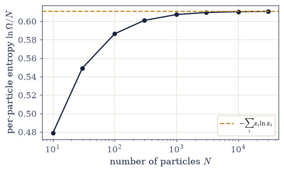
Fig. 411 From a count to an entropy. The per-particle log-multiplicity \(\ln\Omega/N\) for a mixture with \(x_A=0.3\) (dark dots) climbs toward the entropy of mixing \(-\sum_i x_i\ln x_i=0.611\) (dashed) as \(N\) grows: the sub-leading Stirling terms, which scale as \(\ln N/N\), vanish per particle, leaving an extensive entropy. This is \(S=k\ln\Omega\), the first formula of statistical mechanics, and the point where counting, probability, and the large-\(N\) limit become physics.#
Exercise 8 — The most probable macrostate dominates (student)#
We can now see, in one picture, why equilibrium is what it is. For \(N\) coins (or spins), the number of microstates with \(k\) heads is the multiplicity \(\Omega(k)=\binom{N}{k}\), sharply peaked at \(k=N/2\) Eq. 396. As \(N\) grows the peak does not merely stay put — it narrows, with a relative width \(\propto1/\sqrt N\), so an ever-larger fraction of all microstates piles up within a hair of \(k=N/2\) (Fig. 412). At macroscopic \(N\) the states even slightly away from the peak are so vastly outnumbered that they are never observed. This is the whole content of equilibrium: the macrostate we call equilibrium is simply the one realised by the overwhelming majority of microstates, and at large \(N\) it is effectively the only one. The second law is this counting fact at scale. Note that the ratio \(\Omega(k)/\Omega_{\max}\) cannot be formed directly at these \(N\), since both numerator and denominator overflow long before their ratio does. It has to be obtained by subtracting logarithms and exponentiating only at the end.
Part a) Write log_binomial(N, k), the log-multiplicity
\(\ln\binom{N}{k}=\ln N!-\ln k!-\ln(N-k)!\), with every term a scipy.special.gammaln, so that
it is finite for any \(N\) and vectorizes over an array of \(k\). Write this one yourself —
the implementation is the lesson.
Part b) For \(N=100,1000,10000\) form the normalized multiplicity \(\Omega(k)/\Omega_{\max}\) over \(k=0,\dots,N\) by exponentiating \(\ln\Omega(k)-\max_k\ln\Omega(k)\), then read off where it peaks and compute the standard deviation \(\sigma\) of the distribution it defines. Plot the three curves against the fraction \(k/N\) on one axis.
Part c) Confirm that the peak sits at \(k=N/2\) and that the relative width \(\sigma/N\) shrinks as \(1/\sqrt N\), so that any fixed relative window about the peak eventually holds essentially every microstate.
N=100   : peak at k=50 (N/2=50), relative width σ/N = 0.0500
N=1000  : peak at k=500 (N/2=500), relative width σ/N = 0.0158
N=10000 : peak at k=5000 (N/2=5000), relative width σ/N = 0.0050

relative width × √N (∝ constant): [0.5 0.5 0.5]
Validation 8#
✓ the most probable macrostate (k=N/2) dominates: the multiplicity peak narrows as 1/√N
True
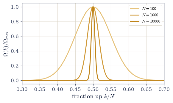
Fig. 412 The multiplicity \(\Omega(k)/\Omega_{\max}=\binom{N}{k}/\binom{N}{N/2}\) against the fractional magnetization \(k/N\), for \(N=100,1000,10000\) (lightening with \(N\)). The peak at \(k=N/2\) sharpens as \(1/\sqrt N\): at large \(N\) essentially every microstate has \(k\) within a vanishing relative window of \(N/2\). Equilibrium is just the macrostate with the most microstates, and at macroscopic \(N\) it is effectively the only one observed — the statistical content of the second law.#
Exercise 9 — The arsenal becomes physics#
Stand back and see the whole arc. We set out three notebooks ago simply to count — socks, poker hands, balls in boxes (§5.1). We turned counts into probabilities and defined the expectation and variance that quantum mechanics will reuse verbatim (§5.2). And here, in the large-\(N\) limit, the mathematics has become physics. Factorials forced us into log space, where Stirling turns a count into an entropy; the central limit theorem explained why the Gaussian is everywhere; and the \(1/\sqrt N\) collapse of fluctuations revealed why a system of \(10^{23}\) parts has sharp, deterministic macroscopic properties at all. The first formula of statistical mechanics, \(S=k\ln\Omega\), fell out of a binomial coefficient and Stirling’s approximation. We set out to count, and we have arrived at entropy.
The three pillars have to agree where they meet, and there is one number where they all do. The per-particle entropy of an evenly mixed system, \(\ln\Omega/N\) at \(x_A=x_B=\tfrac12\), is \(\ln 2\): the same \(\ln 2\) that is the per-spin entropy of a two-state system and the information carried by one bit. Counting, probability, and the large-\(N\) limit are one subject.
Part a) With the log_multiplicity you wrote in Exercise 7, compute the per-particle
log-multiplicity of an evenly split system of \(N=20000\) particles.
Part b) Confirm it equals \(\ln 2\).
per-particle entropy of an evenly mixed system (N=20000): 0.69289
ln 2 = 0.69315   (the entropy of one fair two-state choice — one bit)
counting (§5.1) + probability (§5.2) + the large-N limit (§5.3) = the language of statistical mechanics
Validation 9#
✓ the even-mixing entropy per particle is ln 2 — counting, probability, and large-N meet [got 0.692888 vs expected 0.693147 (rtol=0.001, atol=1e-09)]
True
Notebook summary#
This notebook closes Volume V’s mathematical arsenal by taking counting and probability to the limit statistical mechanics lives in, and handing off to the physics.
The factorial wall Eq. 392: \(1000!\) overflows a float, so we work with \(\ln N!=\)
scipy.special.gammaln\((N+1)\) — statistical mechanics lives in log space (the §0.1 callback).Stirling Eq. 393: \(\ln N!\approx N\ln N-N\) (corrected \(+\tfrac12\ln 2\pi N\)), relative error \(\sim0.9\%\) at \(N=100\) and a few parts in \(10^{6}\) corrected — the analytic handle that turns a count into a closed form.
The limit theorems Eq. 394, Eq. 395: the sample mean converges (law of large numbers); the sum of \(N\) uniforms goes Gaussian by \(N\approx30\) (skew, kurtosis \(\to0\)), and the binomial\((100,\tfrac12)\) matches a Gaussian to \(2\times10^{-4}\) (de Moivre–Laplace).
Sharpness Eq. 396: \(\sigma/\mu=1/\sqrt N\), about \(1.3\times10^{-12}\) at Avogadro’s number — why a mole of gas has a sharp temperature and thermodynamics is deterministic.
The bridge to physics Eq. 397: \(\ln\Omega/N\to-\sum_i x_i\ln x_i\) via Stirling, the entropy of mixing; \(S=k\ln\Omega\) is the first formula of statistical mechanics; and the multiplicity peaks so sharply at \(k=N/2\) that the most probable macrostate is the only one observed — the second law as a counting fact.
We set out to count, and we arrived at entropy. The physics starts at §5.4: microstates, the Boltzmann distribution, and temperature and entropy emerging from the counting built here.
Outlook#
Statistical mechanics proper (§5.4 onward). Microstates, ensembles, the Boltzmann distribution, and temperature and entropy from counting — the physics the arsenal was built for.
Monte Carlo and molecular dynamics. The computational engines of the volume, building on the simulation spine of §5.1–§5.3.
The thermodynamic limit and phase transitions. Where the \(1/\sqrt N\) sharpness can break down — at a critical point fluctuations grow and span all scales (a pointer).
Quantum statistics (Volume VII). The same counting of §5.1, now for indistinguishable particles, giving the Fermi–Dirac and Bose–Einstein distributions.
Cross-reference §0.1 (floating point), §5.1 (counting), and §5.2 (probability).