5.11 A Taste of Non-Equilibrium: Irreversibility, the Arrow of Time, and the Approach to Equilibrium

Elementary Computational Physics

Volume V — Classical Statistical Mechanics Notebook 5.11

The question every ensemble quietly assumed. Microscopic dynamics runs equally well backwards and returns to its start, yet a gas spreads, heat flows, and entropy rises — once. We watch irreversibility emerge from reversible rules in a ring of flipping balls, see a gas find the Maxwell–Boltzmann law, and meet Brownian motion and the Einstein relation. This is a glimpse through a door into a subject of its own; we open it just wide enough to see in.

Level · advanced   •   Est. · 220–260 min

Raymond Amador v1.4.0  ·  2026-07-31  ·  CC BY 4.0 (text) / MIT (code)

Notebook overview

A frank word at the outset, because this notebook is unlike the others. It is the longest and most demanding of the volume, and deliberately so — and it is, we think, among the most rewarding of the whole series. The reason is honest scope: non-equilibrium statistical mechanics is genuinely a subject of its own, several courses’ worth, and we do not attempt a survey. We attempt a single coherent taste. The title word is load-bearing. We will follow one thread — irreversibility, the arrow of time — as far as a notebook can honestly take it, and we will name the rest of the field’s great landmarks as horizons, pointing through the door without pretending to walk the whole room. Modelling that honesty, about what one sitting can and cannot do, is part of the lesson.

The thread answers a question the entire volume quietly assumed and never asked. Every ensemble we built — microcanonical, canonical, grand canonical — described equilibrium: where a system ends up. None asked why it goes there. And the puzzle, once you see it, is sharp. The microscopic dynamics is time-reversible (Hamilton’s equations run backwards just as well; Liouville’s theorem of §5.5) and recurrent (Poincaré: a bounded system returns arbitrarily close to any past state). Yet a gas released in a corner spreads to fill its box and never spontaneously gathers back; heat flows from hot to cold and not the reverse; entropy rises in one direction. How can a temporal asymmetry — an arrow of time — emerge from laws that have none?

The resolution, which we will show rather than assert, is that irreversibility is emergent and probabilistic. It is not in the microscopic laws; it appears when we coarse-grain and count. The Kac ring makes this exactly computable: a deterministic, reversible, periodic toy in which a coarse-grained quantity nonetheless relaxes monotonically — Loschmidt’s reversal and Zermelo’s recurrence objections to Boltzmann, made concrete and answered in a single model. A gas of colliding particles then shows Boltzmann’s H-theorem in action, relaxing irreversibly to the very Maxwell–Boltzmann law of §5.6. And the deep reason is the one that has run through the whole volume: the equilibrium macrostate is overwhelmingly the most probable (the \(1/\sqrt N\) concentration of §5.3), so a system started elsewhere almost certainly moves toward it, while the reversed, entropy-decreasing trajectories — which genuinely exist — are vanishingly rare, and the recurrence times, though real, are longer than the age of the universe by unimaginable factors.

We end with a first taste of transport — Brownian motion, the Langevin equation, and the Green–Kubo relation — which is the dynamical face of the fluctuation–response idea of §5.9. There, §5.9 told us a response function is a static fluctuation; here a transport coefficient turns out to be an equilibrium time correlation, and the Einstein relation \(D=kT/\gamma\) ties diffusion to friction as two faces of the same molecular collisions. The loop closes: the non-equilibrium dynamics relaxes to exactly the Boltzmann equilibrium the rest of the volume described. We began the volume by counting microstates; we end it by watching the arrow of time turn out to be a count.

How to read the checks. Each exercise closes with a validate call against an independent fact: a reversible trajectory retracing itself; the Kac ring relaxing as \((1-2\mu)^t\) and then recurring exactly at \(t=2N\); the Maxwell–Boltzmann distribution minimizing \(H\); a gas relaxing to it with \(H\) monotone; equilibrium’s overwhelming probability and astronomical recurrence; free Brownian motion with \(\langle x^2\rangle=2Dt\) and \(D=kT/\gamma\); the velocity autocorrelation integrating (Green–Kubo) to that same \(D\); and a trapped particle relaxing to \(\langle x^2\rangle =kT/k\). A ✓ is strong evidence; a ✗ is a prompt to locate the discrepancy.

Scope — a taste, and the horizons. One thread (irreversibility) is developed in full; the rest of non-equilibrium statistical mechanics is named, not derived — the full Boltzmann transport equation, the Green–Kubo relations for viscosity and conductivity, Onsager reciprocity, linear response and the dynamical fluctuation–dissipation theorem, the Fokker–Planck and master equations, hydrodynamics, and the modern fluctuation theorems (Jarzynski, Crooks). The production craft of stochastic simulation belongs to molecular-simulation courses and MMM. See Kac (1959); Kardar, Statistical Physics of Particles; Chandler; Zwanzig, Nonequilibrium Statistical Mechanics; and Notebooks §5.5 (Liouville, reversibility), §5.6 (Maxwell–Boltzmann), §5.3 (\(1/\sqrt N\)), §5.4 (the Boltzmann equilibrium), §5.9 (fluctuation–response).

Theory in brief

The puzzle: irreversibility from reversible laws

The microscopic dynamics is time-reversible and recurrent,

(440)\[\text{reverse all velocities} \Rightarrow \text{the system retraces its path};\qquad \text{Poincaré: it returns arbitrarily close to any past state,}\]

yet macroscopic systems approach equilibrium irreversibly and entropy rises in one direction. How a temporal asymmetry emerges from time-symmetric laws is the founding question of non-equilibrium statistical mechanics — the one the equilibrium theory of §5.4–§5.10 never asked.

The Kac ring: irreversibility made exactly computable

\(N\) balls (black or white) sit on a ring; stationary markers occupy a fraction \(\mu\) of the edges. Each step every ball steps one site and flips colour iff it crosses a marker. The dynamics is deterministic, reversible, and periodic (period \(2N\): after two circuits every marker is crossed twice, restoring every colour — Poincaré recurrence, exactly). Yet under the molecular-chaos assumption (treat the markers a ball is about to meet as a random fraction \(\mu\)), the order parameter \(\Delta=\frac1N\sum_i\sigma_i\) relaxes monotonically,

(441)\[\Delta(t)=(1-2\mu)^t\,\Delta(0)\ \to\ 0\ \text{(relaxation)},\qquad \Delta(2N)=\Delta(0)\ \text{(recurrence)} .\]

The same model shows irreversible relaxation (coarse-grained, probabilistic) and exact reversibility/recurrence — Loschmidt and Zermelo, answered: irreversibility is emergent and approximate, not fundamental.

The Boltzmann equation and the H-theorem

Boltzmann’s kinetic equation evolves a gas’s velocity distribution \(f(\mathbf v,t)\) under collisions. Its decisive input is the Stoßzahlansatz (molecular chaos): colliding particles are uncorrelated before they collide. That assumption — not the microscopic dynamics — breaks time-reversal symmetry, and from it follows the H-theorem,

(442)\[H=\int f\ln f\,d\mathbf v\ \text{ decreases monotonically until } f=f_{\rm MB},\]

the entropy \(-kH\) rising to its maximum at the unique stationary state, Maxwell–Boltzmann. The full collision integral and transport equation are named, not derived (a horizon).

Relaxation to Maxwell–Boltzmann

We demonstrate the H-theorem with a caricature of the Boltzmann equation: repeated random binary collisions that conserve momentum and energy (rotate each colliding pair’s relative velocity by a random angle — molecular chaos made literal). From a non-equilibrium start the speed distribution relaxes to the two-dimensional Maxwell–Boltzmann law (§5.6),

(443)\[f(v)=\frac{m}{kT}\,v\,e^{-mv^2/2kT},\qquad H\ \text{monotone decreasing,}\]

and the equilibrium it finds is exactly the Boltzmann distribution of §5.4/§5.6.

The resolution of the paradoxes

Irreversibility does not contradict reversibility; it emerges from coarse-graining + overwhelming probability,

(444)\[\frac{\#\,\text{equilibrium microstates}}{\#\,\text{all microstates}}\to1,\qquad t_{\rm recurrence}\sim e^{O(N)} .\]

The equilibrium macrostate occupies almost all of phase space (the \(1/\sqrt N\) concentration of §5.3), so a system almost certainly moves toward it; reversed trajectories exist but are vanishingly rare, and recurrence times, though real, are astronomically long. The arrow of time is the statistics of large numbers applied to dynamics.

A taste of transport: Brownian motion and Green–Kubo

A heavy particle in a fluid obeys the Langevin equation \(m\,\dot v=-\gamma v+\xi(t)\) with \(\langle\xi(t)\xi(t')\rangle=2\gamma kT\,\delta(t-t')\) — friction and noise are two faces of the same collisions (Einstein 1905). Free Brownian motion diffuses, \(\langle x^2\rangle=2Dt\), with the Einstein relation \(D=kT/\gamma\). The velocity autocorrelation function \(C(t)=\langle v(0)v(t)\rangle\) — how long a fluctuating quantity remembers itself — and the Green–Kubo relation give the transport coefficient as its time integral,

(445)\[C(t)=\frac{kT}{m}e^{-(\gamma/m)t},\qquad D=\int_0^\infty\!\langle v(0)v(t)\rangle\,dt=\frac{kT}{\gamma} .\]

Transport coefficients are equilibrium time-correlation functions — the dynamical fluctuation–dissipation theorem, the time-resolved extension of the static response = fluctuation of §5.9.

The horizons

What this one notebook only peeked at, each a pointer and none developed: the full Boltzmann transport equation and kinetic theory; the Green–Kubo relations for viscosity and thermal conductivity; Onsager’s reciprocal relations; linear response and the dynamical fluctuation–dissipation theorem in full; the Fokker–Planck and master equations; hydrodynamics; and the modern fluctuation theorems (Jarzynski’s \(\langle e^{-\beta W}\rangle=e^{-\beta\Delta F}\), Crooks) relating non-equilibrium work to equilibrium free energy. Non-equilibrium statistical mechanics is a subject of its own; this was a taste.

Setup

The data are the series palette, a red for the ring’s flip markers, and the unit convention \(k_B=1\) (masses, frictions and temperatures are stated per exercise). The one instrument is H_functional, the histogram meter that reads Boltzmann’s \(H\) off a sample of speeds: it fixes the grid so that every distribution in Exercise 4 and every frame of the relaxation in Exercise 5 is measured on the same scale, which is bookkeeping rather than physics. Every dynamics this notebook runs is one of its lessons and is built where it is earned — the reversible velocity-Verlet integrator in Exercise 1, the Kac ring in Exercise 2, the energy-conserving collision update in Exercise 5, the BAOAB Langevin integrator in Exercise 7, and the velocity autocorrelation in Exercise 8. Each exercise seeds its own generator where randomness enters.

The Setup below holds this notebook’s data and instruments — nothing you are asked to build. It is collapsed so the building stays yours; expand it whenever you want the details.

Show code cell source

Hide code cell source

import matplotlib.pyplot as plt
import numpy as np
from matplotlib.animation import FuncAnimation

from ecp import draw, validate
from ecp.animate import show

# data: the series palette, plus a red for the Kac ring's flip markers
ACCENT, INK, SOFT = draw.ACCENT, draw.INK, draw.SOFT
RED = "#c1121f"

# data: units throughout. k_B = 1. Masses, frictions, temperatures stated per exercise.


# instrument: a meter, not a lesson. What Exercises 4 and 5 put under test is which distribution
# minimizes H and that a relaxing gas drives it downhill — not how a sample is binned. The grid is
# fixed here once so every distribution and every frame is measured on the same scale.
def H_functional(speeds, bins=30, v_max=3.5):
    """Boltzmann's H = ∫ f ln f dv, estimated from a speed sample by histogram (`numpy.histogram`).

    Forms the normalized speed density f on a fixed grid and returns Σ_i f_i ln f_i Δv
    over the occupied bins — the discretized ∫ f ln f. The H-theorem says this decreases as a
    gas relaxes, reaching its minimum at the Maxwell–Boltzmann distribution.

    Parameters
    ----------
    speeds : numpy.ndarray
        Particle speeds.
    bins : int, optional
        Number of histogram bins (default ``30``).
    v_max : float, optional
        Upper edge of the speed grid (default ``3.5``).

    Returns
    -------
    float
        The estimated H.
    """
    f, edges = np.histogram(speeds, bins=bins, range=(0.0, v_max), density=True)
    dv = edges[1] - edges[0]
    nz = f > 0
    return float(np.sum(f[nz] * np.log(f[nz])) * dv)

Exercise 1 — The puzzle of the arrow of time (worked)

We begin by sharpening the paradox until it is undeniable. The microscopic laws of motion have no preferred direction of time: run Hamilton’s equations backwards and they are still Hamilton’s equations, and Liouville’s theorem of §5.5 says the flow conserves phase-space volume in either direction. We can see the reversibility directly. Take a particle in some potential, integrate its motion with a time-symmetric (velocity-Verlet) scheme, then reverse its velocity and integrate again — it retraces its path exactly, arriving back where it started Eq. 440 (Fig. 459). And the dynamics is recurrent: Poincaré proved that a bounded system returns arbitrarily close to any earlier state, given enough time. So at the level of the molecules, nothing distinguishes forward from backward, and nothing is lost forever. Yet the world we see is emphatically one-directional — gases spread, cream mixes into coffee, things cool, and never the reverse. The whole equilibrium theory of this volume described the destination without ever asking why the journey runs only one way. That question is the subject of this notebook.

The specimen is a single particle under the anharmonic restoring force \(F(x)=-x-0.3x^3\), whose cubic stiffening keeps the motion from being a special integrable case, started at \(x=1.5\) with \(v=0.4\) and integrated with timestep \(\Delta t=0.01\). Velocity Verlet is the scheme to use because it is time-symmetric: one step advances \(x\to x+v\Delta t+\tfrac12a\Delta t^2\), recomputes the acceleration at the new position, and then advances \(v\to v+\tfrac12(a_{\rm old}+a_{\rm new})\Delta t\), and running that step with the velocity reversed undoes it exactly. Reversibility is therefore a property of the integrator as much as of the physics, and a scheme without it would blur the very point being made.

Part a) Write verlet(x, v, force, dt, n_steps, m=1.0), taking one velocity-Verlet step at a time and returning the final position, the final velocity, and the array of positions visited. Write this one yourself — the implementation is the lesson.

Part b) Integrate \(2000\) steps forward from \((x,v)=(1.5,0.4)\), then reverse the velocity and integrate \(2000\) steps again, and confirm the particle returns to its exact starting point (atol=1e-6) — the microscopic dynamics is time-reversible.

the microscopic dynamics is time-reversible:
  start:                       x = 1.5, v = 0.4
  after forward + velocity-reversed: x = 1.500000, v = 0.400000
  returned to the start: True
yet macroscopic systems never run backwards — that is the puzzle

Validation 1

✓  reversing the velocities retraces the trajectory exactly — the microscopic dynamics is time-reversible (yet macroscopic behavior is not)   [max|Δ| = 8.77076e-15 (rtol=1e-06, atol=1e-06)]

True

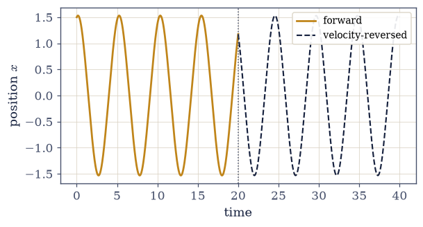
Fig. 459 The microscopic dynamics is time-reversible. A particle in an anharmonic potential is integrated forward (amber) with a time-symmetric velocity-Verlet scheme; at the end its velocity is reversed and it is integrated again (dark, dashed), retracing its path exactly back to the start. Hamilton’s equations have no preferred direction of time, and (Poincaré) a bounded system even returns arbitrarily close to any past state. Nothing at the level of the molecules distinguishes forward from backward — which is precisely why the one-directional world we actually see, where gases spread and entropy rises, is a puzzle the rest of this notebook resolves.

Exercise 2 — The Kac ring I: irreversible relaxation under molecular chaos (worked)

To resolve the puzzle we need a model simple enough to understand completely and rich enough to show the paradox, and Mark Kac’s ring (1959) is the perfect one. Picture \(N\) balls on a ring of \(N\) sites, each ball black or white, and fix markers on some fraction \(\mu\) of the edges between sites (Fig. 460). The rule: at every step each ball advances one site, and it flips colour if and only if it crosses a marker. The markers never move; only the balls circulate. This dynamics is utterly deterministic and, as we will see in Exercise 3, exactly reversible and periodic — there is no randomness and no friction anywhere in it. And yet watch the order parameter \(\Delta=\frac1N\sum_i\sigma_i\) (the excess of one colour). If we make the molecular-chaos assumption — that the markers a ball is about to encounter are a random fraction \(\mu\) of the edges ahead, uncorrelated with its history — then each step a fraction \(\mu\) of balls flip, and a short calculation gives monotonic, irreversible relaxation, \(\Delta(t)=(1-2\mu)^t\Delta(0)\to0\) Eq. 441. The coarse-grained quantity decays to equilibrium exactly as the H-theorem will have a gas do — and from a perfectly reversible rule.

Coding the ring is three lines and one trap. Represent the balls as \(\sigma_i=\pm1\) and the edges as \(\eta_i=\pm1\), with \(\eta_i=-1\) on the fraction \(\mu\) of edges that carry a marker; then one step of the whole ring is \(\sigma\leftarrow\eta\cdot\mathrm{roll}(\sigma,1)\), a circulation by one site (numpy.roll) followed by a flip wherever a marker was crossed. The trap is that the markers are placed once and never move again — it is the balls that circulate past them, and a version that rolls the markers too is a different (and unremarkable) model. The run below uses \(N=4000\) balls and \(\mu=0.12\): the molecular-chaos prediction is exact only as \(N\to\infty\), so a large ring keeps the early agreement tight, and the first eight steps are the window where the markers ahead of a ball really are uncorrelated with its history.

Part a) Write kac_ring(N, mu, n_steps, rng), which starts every ball white (\(\sigma_i=+1\), so \(\Delta(0)=1\)), places the markers once with rng, and returns the order-parameter trace \(\Delta(t)=\frac1N\sum_i\sigma_i\) of length n_steps + 1. Write this one yourself — the implementation is the lesson.

Part b) Run it for \(2N\) steps and confirm the early relaxation matches the molecular-chaos prediction \((1-2\mu)^t\) over the first eight steps (atol=5e-2), and that \(\Delta\) then sits near zero.

Kac ring: N = 4000 balls, μ = 0.12 (fraction of marked edges)
  early relaxation vs molecular-chaos (1−2μ)^t:
    Δ(1) = +0.7535   (1−2μ)^t = +0.7600
    Δ(3) = +0.4575   (1−2μ)^t = +0.4390
    Δ(5) = +0.2795   (1−2μ)^t = +0.2536
  Δ falls toward 0: typical |Δ| in the relaxed window ≈ 0.0248

Validation 2

✓  under molecular chaos the Kac-ring order parameter relaxes as (1−2μ)^t — irreversible decay from a reversible rule   [max|Δ| = 0.0273782 (rtol=1e-06, atol=0.05)]

True

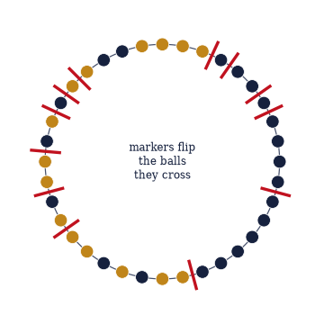
Fig. 460 The Kac ring. \(N\) balls (amber/ink for the two colours) circulate one site per step around a ring whose edges carry fixed markers (red ticks) on a fraction \(\mu\) of them; a ball flips colour whenever it crosses a marker. The markers are stationary — only the balls move. Nothing in the rule is random or dissipative, and (Exercise 3) the dynamics is exactly reversible and periodic. Yet under the molecular-chaos assumption the colour imbalance \(\Delta\) relaxes monotonically to zero, the H-theorem in miniature — irreversibility manufactured from a reversible rule, which is the whole paradox in one toy.

Exercise 3 — The Kac ring II: reversibility, recurrence, and the paradoxes resolved (worked)

Now we spring the trap that caught Boltzmann’s critics, and disarm it. Boltzmann claimed his gas relaxes irreversibly to equilibrium; two objections followed. Loschmidt (the reversal paradox): the laws are time-symmetric, so for every relaxing trajectory there is a reversed one in which entropy decreases — how can relaxation be universal? Zermelo (the recurrence paradox): Poincaré says a bounded system returns to its start, so entropy cannot rise forever. The Kac ring settles both, because we can compute its exact dynamics, not just the molecular-chaos approximation. Run the ring out to \(t=2N\) and the order parameter \(\Delta\) snaps exactly back to \(\Delta(0)\) (Fig. 461): after two full circuits every ball has crossed every marker exactly twice, two flips cancel, and the original configuration is restored, period \(2N\) Eq. 441. And the dynamics is reversible — reverse the stepping and it retraces. So both objections are correct: the exact dynamics is reversible and recurrent. They simply do not contradict the relaxation, because the smooth \((1-2\mu)^t\) decay was never the exact dynamics — it was the molecular-chaos approximation, which holds early (when the markers ahead really are uncorrelated with a ball’s history) and breaks down long before the recurrence. Irreversibility is emergent and approximate, exact at neither the shortest nor the recurrence timescale. Loschmidt and Zermelo, answered in one model.

The trace already computed in Exercise 2 ran to \(t=2N\), so both recurrences are in it and nothing new needs simulating. Two entries tell the story: the half-period value \(\Delta(N)\), where every ball has crossed every marker exactly once and the sign of \(\Delta\) is simply flipped for a ring with an odd number of markers, and the full-period value \(\Delta(2N)\), where every marker has been crossed twice and the two flips cancel. Neither is approximate, which is why the check below can demand a relative tolerance of \(10^{-9}\) rather than the loose tolerance a statistical claim would need.

Part a) From the \(\Delta(t)\) trace of the kac_ring you wrote in Exercise 2, read off \(\Delta(0)\), the half-period value \(\Delta(N)\), and the full-period value \(\Delta(2N)\).

Part b) Confirm \(\Delta(2N)=\Delta(0)\) to rtol=1e-9 — exact Poincaré recurrence, with the molecular-chaos curve of Exercise 2 having tracked only the early relaxation.

Kac ring exact dynamics (N = 4000):
  Δ(0)  = +1.0000
  Δ(N)  = -1.0000   (half-period recurrence (-1)^m Δ(0) = ±1, not chaos's ≈0)
  Δ(2N) = +1.0000   ← exact recurrence to Δ(0) (Poincaré/Zermelo, period 2N)
the smooth (1−2μ)^t decay was the molecular-chaos approximation, not the reversible exact dynamics

Validation 3

✓  the exact Kac-ring dynamics recurs at t=2N (Poincaré) — reversible and recurrent underneath the irreversible relaxation   [got 1 vs expected 1 (rtol=1e-09, atol=1e-09)]

True

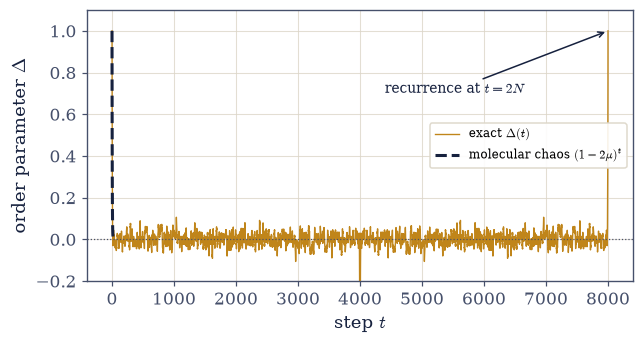
Fig. 461 Irreversible relaxation and exact recurrence in one model. The Kac-ring order parameter \(\Delta(t)\) over two full circuits (amber). Early on it relaxes monotonically toward zero, tracking the molecular-chaos prediction \((1-2\mu)^t\) (dark dashed) — the H-theorem in miniature. It then fluctuates near zero for a long plateau, and at \(t=2N\) snaps exactly back to \(\Delta(0)=1\): Poincaré recurrence, the dynamics revealed as reversible and periodic all along. Loschmidt’s reversal and Zermelo’s recurrence objections are both correct and both harmless — the smooth decay was only an approximation, valid early and broken long before the recurrence. Irreversibility is emergent, not fundamental.

Exercise 4 — The H-theorem and the Stoßzahlansatz (worked)

With the Kac ring’s lesson in hand, we name the real thing it models. Boltzmann’s kinetic equation describes how a gas’s velocity distribution \(f(\mathbf v,t)\) evolves under collisions, and its crucial input is the Stoßzahlansatz — the molecular-chaos assumption that two particles about to collide are uncorrelated, exactly the assumption that made the markers “random” in the Kac ring. That assumption, and not the underlying reversible mechanics, is what breaks time-reversal symmetry, and from it Boltzmann proved his H-theorem: the functional \(H=\int f\ln f\,d\mathbf v\) decreases monotonically (so the entropy \(-kH\) increases) until \(f\) reaches the unique stationary distribution Eq. 442. That stationary distribution is Maxwell–Boltzmann — and we can see why it is special directly: among all velocity distributions with a fixed energy, Maxwell–Boltzmann is the one that minimizes \(H\) (equivalently, maximizes entropy), so any other same-energy distribution sits higher and the H-theorem drives the gas downhill to it. The full collision integral and the Boltzmann transport equation that surrounds it are a horizon we name but do not derive.

Reading \(H\) off a finite sample is a measurement, and the Setup’s H_functional is the meter: it bins the speeds on a fixed grid, normalizes to a density \(f\), and sums \(f_i\ln f_i\,\Delta v\) over the occupied bins — the discretized \(\int f\ln f\,dv\), with empty bins left out because \(f\ln f\to0\) there. The grid is the same (\(30\) bins over \(0\le v\le3.5\)) for everything measured in this notebook, since a comparison made on two different grids would measure the binning instead of the physics. The three test distributions each carry \(40\,000\) two-dimensional velocities at the same mean kinetic energy \(\langle v^2\rangle=1\): Maxwell–Boltzmann with \(kT/m=0.5\) (each component a Gaussian of variance \(kT/m\)), a set with every particle at the same speed \(v_{\rm rms}\) in a random direction, and a two-speed mixture (\(v_{\rm rms}/2\) and \(\sqrt{1.5}\,v_{\rm rms}\), half the particles each).

Part a) Build those three equal-energy samples with numpy.random.default_rng.

Part b) Compute \(H\) for each and confirm Maxwell–Boltzmann has the lowest — the equilibrium the H-theorem drives toward.

H = ∫ f ln f for three distributions at the same energy ⟨v²⟩ = 1:
  Maxwell–Boltzmann : H = -0.597   ← the minimum (maximum entropy)
  all equal speed   : H = +2.148
  two speeds        : H = +1.455

Validation 4

✓  the Maxwell–Boltzmann distribution has lower H than the tested non-equilibrium distributions — the equilibrium the H-theorem drives toward

True

Exercise 5 — A gas relaxes to Maxwell–Boltzmann (worked)

Now we watch the H-theorem happen. We model a gas by a caricature of the Boltzmann collision process: repeated random binary collisions that conserve momentum and energy, each one rotating a colliding pair’s relative velocity by a random angle. This is molecular chaos made literal — every collision scrambles the participants’ correlations — and it is exactly the ingredient that makes the dynamics irreversible. We start the gas in a sharply non-equilibrium state, all particles moving at the same speed in random directions, and let the collisions run. The speed distribution flows, irreversibly, to the two-dimensional Maxwell–Boltzmann law \(f(v)\propto v\, e^{-mv^2/2kT}\) of §5.6 Eq. 443, and Boltzmann’s \(H=\int f\ln f\) falls monotonically the whole way (Fig. 462). Energy and momentum are conserved at every step, so nothing is driving the gas but the statistics of collisions — and yet it has a clear, one-directional destination. The equilibrium it finds is precisely the Boltzmann distribution the rest of the volume computed from the ensembles; the dynamics and the ensembles agree.

One collision is pure bookkeeping in the centre-of-mass frame. For a pair \((i,j)\) write \(\mathbf v_{\rm cm}=\tfrac12(\mathbf v_i+\mathbf v_j)\) and \(\mathbf v_{\rm rel}=\mathbf v_i-\mathbf v_j\); rotating \(\mathbf v_{\rm rel}\) by an angle \(\theta\) and putting the pair back as \(\mathbf v_{i,j}=\mathbf v_{\rm cm}\pm\tfrac12\mathbf v_{\rm rel}\) leaves the total momentum (through \(\mathbf v_{\rm cm}\)) and the total kinetic energy (through \(|\mathbf v_{\rm rel}|\)) untouched, so nothing but the direction information is scrambled — which is exactly what molecular chaos asserts. The gas below is \(15\,000\) particles started at the single speed \(v_0=1\) in random directions, relaxed in \(50\) rounds of \(3000\) collisions each, with \(H\) and a snapshot of the speeds recorded after every round. In two dimensions the equilibrium it should find has \(\langle v^2\rangle=2kT/m\), mean speed \(\sqrt{\pi kT/2m}\) and \(v_{\rm rms}=\sqrt{2kT/m}\).

Part a) Write random_collisions(v, n_collisions, rng), applying that many random binary collisions to a velocity array of shape (n, 2) in place and returning it. Write this one yourself — the implementation is the lesson.

Part b) Relax the gas from its all-equal-speed start, recording \(H\) (with the Setup’s H_functional, on the same grid Exercise 4 used) and the speed distribution after each round of collisions.

Part c) Confirm the final mean and rms speeds match the 2-D Maxwell–Boltzmann values (rtol=2e-2), that \(H\) fell monotonically, and that the kinetic energy was conserved throughout. The animation shows the distribution morphing to Maxwell–Boltzmann.

gas relaxation by energy-conserving collisions (n = 15000):
  H decreased: +2.148 → -0.604  (monotone: True)
  kinetic energy conserved: True
  ⟨|v|⟩ = 0.8844 vs MB √(πkT/2m) = 0.8862;  v_rms = 1.0000 vs √(2kT/m) = 1.0000

Validation 5

✓  energy-conserving collisions relax the gas to the 2-D Maxwell–Boltzmann distribution (5.6)   [max|Δ| = 0.00179839 (rtol=0.02, atol=1e-09)]
✓  H = ∫ f ln f decreases monotonically as the gas relaxes — the H-theorem in action

True

Once Loop Reflect

Fig. 462 A gas relaxing to Maxwell–Boltzmann (animated), the H-theorem in action. Starting from a sharply non-equilibrium state (all particles at one speed), energy- and momentum-conserving random collisions drive the speed distribution (amber histogram) to the two-dimensional Maxwell–Boltzmann law \(f(v)\propto v\,e^{-mv^2/2kT}\) (dark curve, 5.6). Inset: Boltzmann’s \(H=\int f\ln f\) falls monotonically throughout — the entropy \(-kH\) rising to its maximum. Nothing drives the gas but the statistics of collisions, energy is conserved at every step, yet the relaxation is unmistakably one-directional. The equilibrium it finds is exactly the Boltzmann distribution the ensembles of this volume computed.

Exercise 6 — The resolution: irreversibility as overwhelming probability (worked)

We can now state the resolution plainly, because every piece is in place. Irreversibility does not contradict the reversibility of the microscopic laws; it emerges from coarse-graining plus overwhelming probability, and the overwhelming probability is the same \(1/\sqrt N\) concentration that has run through the whole volume Eq. 444. The equilibrium macrostate corresponds to so vastly many more microstates than any non-equilibrium one (§5.3, §5.4) that it occupies essentially all of phase space; a system started in a rare, ordered corner therefore moves, with overwhelming probability, toward equilibrium — not because it is forced to, but because almost every path leads there. The reversed, entropy-decreasing trajectories that Loschmidt invoked genuinely exist, but they are a vanishing fraction, and the Poincaré recurrences that Zermelo invoked are real but occur on timescales of order \(e^{N}\). Put a number on it: for a macroscopic gas of \(N\sim10^{23}\) particles the recurrence time exceeds the age of the universe not by a large factor but by a factor of order \(10^{(10^{23})}\) — a number whose exponent dwarfs every quantity in cosmology. The arrow of time is not a new law layered onto mechanics; it is the statistics of large numbers applied to dynamics, the same sharpness that made macrostates definite in §5.3 now making time’s direction effectively absolute.

The estimate needs only three numbers and one exponent. A macroscopic sample holds \(N\approx6\times10^{23}\) particles, its microscopic clock is a collision time of about \(10^{-13}\,\)s, and the universe is some \(4.4\times10^{17}\,\)s old. Poincaré recurrence takes of order \(e^{N}\) microscopic times, so the ratio of the recurrence time to the age of the universe is best handled in logarithms: \(\log_{10}=N/\ln10-\log_{10}(t_{\rm universe}/t_{\rm micro})\), where the second term — about \(30\) — is utterly swamped by the first.

Part a) Form that \(\log_{10}\) of the recurrence time in units of the age of the universe.

Part b) Confirm it exceeds \(10^{20}\): recurrence and reversal are real but utterly negligible, so the arrow of time is effectively absolute.

the resolution: equilibrium is overwhelmingly probable; recurrence is real but negligible
  Poincaré recurrence time / age of universe ≈ 10^(2.61e+23)
  i.e. the recurrence time is ~10^(10^23) times the age of the universe — utterly unobservable
  reversed (entropy-decreasing) paths exist but are a vanishing fraction ~e^(−O(N)) of all paths

Validation 6

✓  equilibrium is overwhelmingly probable and the recurrence time is astronomical (~e^N) — reversal and recurrence are real but negligible, so the arrow of time is effectively absolute

True

Exercise 7 — Brownian motion and the Einstein relation (worked)

Having understood why systems relax, we turn to how fast — transport — and take our first honest taste of it through the phenomenon that founded the subject. A pollen grain in water jitters ceaselessly, kicked by the molecules it cannot see; Einstein (1905) and Langevin (1908) modelled this as a heavy particle obeying \(m\,\dot v=-\gamma v+\xi(t)\), where the same molecular collisions appear twice — as a systematic friction \(-\gamma v\) and as a randomly fluctuating force \(\xi\) with \(\langle\xi(t)\xi(t')\rangle=2\gamma kT\,\delta(t-t')\) Eq. 445. That the friction coefficient and the noise strength are locked together by the same \(\gamma kT\) is the first fluctuation–dissipation relation: dissipation (friction) and fluctuation (noise) are two faces of one molecular reality. Its most famous consequence is that free Brownian motion diffuses, \(\langle x^2\rangle=2Dt\), with the Einstein relation \(D=kT/\gamma\) (Fig. 463) — the diffusion constant (a fluctuation) fixed by the friction (a dissipation), the dynamical extension of the static response = fluctuation of §5.9. We integrate the Langevin equation with the BAOAB scheme, whose accuracy we will need in the next exercise.

BAOAB is a splitting: the Langevin equation is broken into three pieces that can each be advanced exactly or symmetrically, and one timestep applies them in the palindromic order B–A–O–A–B. B is half a force kick, \(v\to v+\tfrac12\Delta t\,F(x)/m\) with \(F=-k_{\rm spring}x\) (zero for a free particle); A is half a drift, \(x\to x+\tfrac12\Delta t\,v\); and O is the Ornstein–Uhlenbeck thermostat, applied exactly rather than by a Taylor step, \(v\to cv+\sqrt{(1-c^2)kT/m}\;\mathcal N(0,1)\) with \(c=e^{-\gamma\Delta t/m}\) — friction and noise entering together, in the ratio the fluctuation–dissipation relation fixes. The palindrome is what makes the scheme accurate on the configurational side, and the exact O step is what makes it sample \(\langle v^2\rangle=kT/m\) correctly; a naive Euler–Maruyama integrator biases that variance and would inflate the Green–Kubo integral of Exercise 8, so the choice is not cosmetic. The run below is \(8000\) independent free particles (\(k_{\rm spring}=0\)) for \(1500\) steps of \(\Delta t=0.02\) at \(m=\gamma=kT=1\), all released from \(x_0=0\) with velocities drawn from the Maxwell–Boltzmann \(\sqrt{kT/m}\,\mathcal N(0,1)\). The mean-square displacement is diffusive only after the ballistic transient, so the slope is fit on \(t>5\) alone.

Part a) Write langevin_baoab(n_part, n_steps, dt, m, gamma, kT, rng, k_spring=0.0, x0=0.0, v_init=None), returning the position and velocity histories (X, V), each of shape (n_steps + 1, n_part). Write this one yourself — the implementation is the lesson.

Part b) Simulate the free Brownian ensemble with it and form the mean-square displacement \(\langle x^2\rangle(t)\) over the particles.

Part c) Fit the diffusive slope on the late-time window, halve it to get \(D\), and confirm the Einstein relation \(D=kT/\gamma\) (rtol=8e-2).

free Brownian motion (m = γ = kT = 1, dt = 0.02):
  diffusion from ⟨x²⟩ = 2Dt:  D = 1.0089
  Einstein relation D = kT/γ: D = 1.0000
  diffusion (a fluctuation) is fixed by friction (a dissipation) — fluctuation–dissipation

Validation 7

✓  free Brownian motion gives ⟨x²⟩ = 2Dt with the Einstein relation D = kT/γ (a fluctuation–dissipation relation)   [got 1.00892 vs expected 1 (rtol=0.08, atol=1e-09)]

True

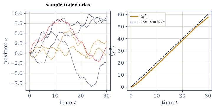
Fig. 463 Brownian motion and the Einstein relation. Left: a few sample Langevin trajectories \(x(t)\) — the erratic wandering of a heavy particle kicked by molecular collisions. Right: the mean-square displacement \(\langle x^2\rangle\) over many particles grows linearly, \(\langle x^2\rangle=2Dt\) (dashed), the signature of diffusion; its slope gives \(D=kT/\gamma\) — the Einstein relation. Friction and noise are the same molecular collisions seen two ways, so the diffusion constant (a fluctuation) is fixed by the friction (a dissipation): the first fluctuation–dissipation relation, and the dynamical extension of the static response = fluctuation of §5.9.

Exercise 8 — Autocorrelation functions and Green–Kubo (worked)

We close the transport taste with the idea that is the modern language of the whole subject, and we build the one new tool it needs from scratch, here where it is used. The tool is the autocorrelation function \(C(t)=\langle A(0)A(t)\rangle\): it measures how long a fluctuating quantity remembers itself, starting at the variance \(\langle A^2\rangle\) at \(t=0\) and decaying over a characteristic correlation time as the memory is lost. For the Brownian particle’s velocity, the velocity autocorrelation function is \(C(t)=\langle v(0)v(t)\rangle=(kT/m)\,e^{-(\gamma/m)t}\), a clean exponential decaying over the time \(m/\gamma\) Eq. 445. The remarkable Green–Kubo relation then expresses the transport coefficient as the time integral of this equilibrium correlation, \(D=\int_0^\infty\langle v(0)v(t)\rangle\,dt=kT/\gamma\) (Fig. 464) — the same \(D\) we got from the mean-square displacement and from Einstein, now as an integral over how the velocity forgets itself. This is the deep, general statement: a transport coefficient is an equilibrium time-correlation function, the dynamical fluctuation–dissipation theorem. One numerical caution, which we honour: we first verify the integrator gives \(\langle v^2\rangle=kT/m\) (an inaccurate scheme biases this and inflates the integral), then integrate the autocorrelation with numpy.trapezoid, truncating after a few correlation times.

Estimating \(C(t)\) from a finite record is an averaging question. A single pair \(v(0)v(t)\) is almost pure noise, so one averages over the particles — the columns of the velocity history — and over many time origins, since in equilibrium every instant is as good a \(t=0\) as any other. With a record of \(n\) rows and n_lag lags wanted, the clean choice is to use the first \(n-\texttt{n\_lag}\) rows as origins and, for each lag \(t\), average the elementwise product of that block with the block shifted forward by \(t\). The trajectories are the Exercise 7 ones, so the same \(m=\gamma=kT=1\) and \(\Delta t=0.02\) apply; \(350\) lags reach about seven correlation times \(m/\gamma\), far enough out that the truncated integral has already flattened, and the first \(500\) steps are dropped from the variance check so the ensemble is thermalized.

Part a) Verify \(\langle v^2\rangle=kT/m\) for the BAOAB trajectories of Exercise 7 (rtol=2e-2) — this comes first, because an inaccurate integrator would quietly inflate everything after it.

Part b) Write vacf(V, n_lag), returning \(C(t)=\langle v(0)v(t)\rangle\) for lags \(0,1,\dots,\texttt{n\_lag}-1\) in timestep units. Write this one yourself — the implementation is the lesson.

Part c) Confirm \(C\) decays as \((kT/m)e^{-(\gamma/m)t}\) from \(C(0)=kT/m\), and integrate it with numpy.trapezoid to recover the Green–Kubo \(D=kT/\gamma\) (rtol=5e-2) — the same \(D\) the mean-square displacement gave.

integrator check: ⟨v²⟩ = 0.9988 vs kT/m = 1.0000  (must hold before trusting Green–Kubo)

velocity autocorrelation C(t) = ⟨v(0)v(t)⟩:
  C(0) = 0.9998 vs kT/m = 1.0000;  decay matches (kT/m)e^(−γt/m) to max |Δ| = 0.0020
  Green–Kubo D = ∫₀^∞ C(t) dt = 0.9999  vs  kT/γ = 1.0000  (agrees with the MSD/Einstein D)
  a transport coefficient IS an equilibrium time-correlation — the dynamical fluctuation–dissipation theorem

Validation 8

✓  the BAOAB integrator gives ⟨v²⟩ = kT/m (verified before trusting the Green–Kubo integral)   [got 0.998755 vs expected 1 (rtol=0.02, atol=1e-09)]
✓  the velocity autocorrelation integrates (Green–Kubo) to the diffusion coefficient D = kT/γ   [max|Δ| = 0.000245462 (rtol=0.05, atol=1e-09)]

True

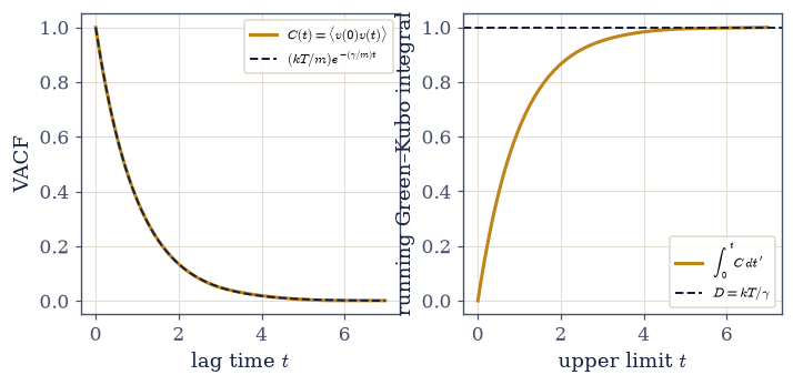
Fig. 464 Green–Kubo: a transport coefficient is an equilibrium time-correlation. Left: the velocity autocorrelation \(C(t)=\langle v(0)v(t)\rangle\) (amber) from the Langevin trajectories, decaying as \((kT/m)e^{-(\gamma/m)t}\) (dark dashed) over the correlation time \(m/\gamma\) — a measure of how long the velocity remembers itself. Right: its running time integral \(\int_0^t C\,dt'\) (amber) rises to the diffusion coefficient \(D=kT/\gamma\) (dashed), the Green–Kubo relation — the same \(D\) obtained from the mean-square displacement and from Einstein. Transport coefficients are equilibrium time-correlation functions: the dynamical fluctuation–dissipation theorem, the time-resolved face of 5.9.

Exercise 9 — The Langevin dynamics relaxes to the Boltzmann equilibrium (student)

Before the synthesis, we close the loop the whole volume has drawn — explicitly, with the dynamics flowing into the ensembles. Put a Brownian particle not in free space but in a harmonic trap, \(U(x)= \tfrac12 k x^2\), and start it far from the bottom. The Langevin dynamics — the same friction and noise — now does two things at once: the friction drains its excess energy and the noise keeps it warm, and the competition settles into a stationary distribution. That distribution is exactly the Boltzmann one, \(P(x)\propto e^{-kx^2/2kT}\), with \(\langle x^2\rangle=kT/k\) — equipartition, the very result the canonical ensemble of §5.8 gave for a harmonic degree of freedom. So the non-equilibrium dynamics does not merely resemble the equilibrium theory; it flows into it. The arrow of time we have been chasing points precisely at the equilibrium distributions the rest of the volume built, and the two descriptions — the dynamics that takes a system there, and the ensemble that describes it once arrived — are one consistent whole.

The trap has stiffness \(k=2\) and the particle starts at rest at \(x_0=3\), far outside the thermal width \(\sqrt{kT/k}\approx0.7\) it must settle into, so the relaxation is visible rather than assumed; \(10\,000\) independent particles are run for \(2500\) steps at the same \(m=\gamma=kT=1\) and \(\Delta t=0.02\) as before. The equilibrium average is taken only after step \(1200\), by which time the transient has decayed and what is left is the stationary state.

Part a) Release the trapped ensemble with the langevin_baoab you wrote in Exercise 7, passing the spring constant, the off-centre start and a zero initial velocity.

Part b) Measure \(\langle x^2\rangle\) over the post-transient part of the run and confirm it equals the Boltzmann/equipartition value \(kT/k\) (rtol=1e-1) — the ensembles’ answer, reached by the dynamics.

trapped Langevin particle (spring k = 2.0, released from x₀ = 3):
  equilibrium ⟨x²⟩ = 0.4996  vs  Boltzmann/equipartition kT/k = 0.5000
  the non-equilibrium dynamics flows into the Boltzmann equilibrium of the ensembles (5.4/5.8)

Validation 9

✓  the trapped Langevin particle relaxes to the Boltzmann equilibrium ⟨x²⟩ = kT/k (equipartition) — the dynamics flows into the ensembles   [got 0.499593 vs expected 0.5 (rtol=0.1, atol=1e-09)]

True

Exercise 10 — A glimpse through the door, and the close of the volume (synthesis)

We have opened the door just wide enough to see that the room behind it is enormous. The equilibrium theory of this volume described where systems rest; this notebook asked how they get there, and found that irreversibility and the arrow of time are not extra laws but emergent facts — they appear, probabilistically, the moment one coarse-grains and counts. The Kac ring made it exact: a reversible, recurrent toy whose coarse-grained order parameter nonetheless relaxes, answering Loschmidt and Zermelo in one model. A gas finding Maxwell–Boltzmann made it physical, the H-theorem driving a non-equilibrium distribution downhill to the very equilibrium the ensembles compute. The resolution named the mechanism: equilibrium is overwhelmingly probable (the \(1/\sqrt N\) of §5.3 once more), recurrences and reversals real but astronomically rare. And Brownian motion, the Einstein relation, and Green–Kubo gave a first taste of transport — diffusion and friction as one molecular reality, a transport coefficient revealed as an equilibrium time-correlation, the dynamical fluctuation–dissipation theorem extending the static one of §5.9 — with the trapped particle flowing back into the Boltzmann equilibrium and closing the loop.

And then the honest horizons, named not crossed: the full Boltzmann transport equation and kinetic theory; the Green–Kubo relations for viscosity and conductivity; Onsager reciprocity; linear response and the fluctuation–dissipation theorem in full; the Fokker–Planck and master equations; hydrodynamics; and the modern fluctuation theorems of Jarzynski and Crooks, which tie non-equilibrium work to equilibrium free energy. Each is a doorway of its own, and non-equilibrium statistical mechanics is a subject of its own. This was a taste.

There is no new computation here: the closing is the result. With it the volume closes. We began at counting — how many microstates realize a macrostate (§5.1) — and built, from probability alone, the entropy, the temperature, the ensembles, the structure of thermodynamics, the emergence of order, and now the arrow of time. The arrow that felt like a fundamental law turned out to be a count: the same statistics of large numbers that opened the volume, now pointing the direction of time itself.

Notebook summary

This final notebook of Volume V took a single honest taste of non-equilibrium statistical mechanics, following irreversibility from reversible microscopic laws and closing the volume.

• The puzzle Eq. 440: the microscopic dynamics is time-reversible (a Verlet trajectory retraces under velocity reversal) and recurrent, yet macroscopic systems relax irreversibly.

• The Kac ring Eq. 441: a reversible, periodic toy whose order parameter relaxes as \((1-2\mu)^t\) under molecular chaos (verified) yet recurs exactly at \(t=2N\) (verified) — Loschmidt’s reversal and Zermelo’s recurrence answered: irreversibility is emergent and approximate.

• The H-theorem Eq. 442, Eq. 443: the Stoßzahlansatz (molecular chaos) breaks time-reversal symmetry; Maxwell–Boltzmann minimizes \(H=\int f\ln f\), and a gas of energy-conserving collisions relaxes to it (verified, \(H\) monotone) — the Boltzmann equilibrium of §5.6.

• The resolution Eq. 444: irreversibility is coarse-graining + overwhelming probability (the \(1/\sqrt N\) of §5.3); recurrence times \(\sim e^N\) dwarf the age of the universe by \(\sim10^{(10^{23})}\).

• A taste of transport Eq. 445: free Brownian motion gives \(\langle x^2\rangle=2Dt\) with the Einstein \(D=kT/\gamma\); the velocity autocorrelation \((kT/m)e^{-(\gamma/m)t}\) integrates (Green–Kubo) to the same \(D\) — transport coefficients are equilibrium time-correlations, the dynamical fluctuation–dissipation theorem (§5.9). A trapped particle relaxes to \(\langle x^2\rangle =kT/k\), the ensembles’ equilibrium.

Volume V built equilibrium from probability and then watched equilibrium assemble itself; the arrow of time, which felt like a law, turned out to be the count that began the volume.

Outlook

• Non-equilibrium statistical mechanics, a subject of its own. The Boltzmann transport equation and kinetic theory; the Green–Kubo relations for viscosity and thermal conductivity; Onsager reciprocity; linear response and the full fluctuation–dissipation theorem; the Fokker–Planck and master equations; hydrodynamics; and the modern fluctuation theorems (Jarzynski, Crooks) — each a horizon, a possible course of its own.

• Stochastic and molecular simulation. The Langevin integrator here is a first step, and §5.17 takes the deterministic one the rest of the way — periodic boundaries, a measured pressure, and honest error bars on a correlated trajectory. §5.18 then watches a metastable state decay, but only where the driving is strong enough that it decays unaided. The production craft that reaches the genuinely rare — canonical thermostats, free-energy methods, umbrella and forward-flux sampling — still belongs to molecular-simulation courses and MMM, and both notebooks say where they stop.

• Volume VII: the quantum arrow of time. Quantum dynamics, the quantum Boltzmann equation, and decoherence — how irreversibility appears in quantum systems — once Volume VI builds the mechanics.

• Cross-reference §5.5 (Liouville, reversibility, ergodicity), §5.6 (Maxwell–Boltzmann), §5.3 (\(1/\sqrt N\)), §5.4 (the Boltzmann equilibrium), §5.9 (the static fluctuation–response this extends).

Take this notebook with you

Use the download button (↓) in the toolbar above to save this notebook and run it yourself. The published notebooks ship without worked solutions; if you would like the reference solutions — to teach from or to check your own work — get in touch: hello@ramador.me.