1.5 Coupled Oscillators and Normal Modes

Elementary Computational Physics

Volume I — Elementary Mechanics Notebook 1.5

Diagonalising the equations of motion: normal modes as an eigenvalue problem, the 1-D chain dispersion relation, and beating as two modes seen in the time domain.

Level · intermediate   •   Est. · 60–90 min

Raymond Amador v1.4.0  ·  2026-07-31  ·  CC BY 4.0 (text) / MIT (code)

Notebook overview

A single mass on a spring oscillates at one frequency. Couple a few of them together and the motion looks hopelessly tangled: each mass pushes its neighbours, which push back. The classical insight is that the tangle is an illusion of the coordinates: in the right basis the system falls apart into independent oscillators called normal modes, each a single frequency and a fixed shape. Finding that basis is nothing more than solving an eigenvalue problem, and once we have it the whole of small-oscillation theory (mode shapes, the dispersion relation of a chain, even the slow beating of two weakly coupled pendulums) follows from linear algebra.

We will (1) assemble the stiffness matrix and solve the mode eigenproblem, (2) read the in-phase and anti-phase mode shapes off the eigenvectors, (3, 4) check the mode frequencies of a three-mass system and a twenty-mass chain against the analytic dispersion relation, (5) integrate the motion in time and use energy conservation as an integrator check, (6) animate a single normal mode oscillating rigidly at one frequency, and (7) animate the beating of two weakly coupled oscillators and recover the beat period.

How to read the checks. Each exercise ends with a validation that compares our result to an expected physical fact. A ✗ does not by itself mean the answer is wrong: it means the output didn’t match what the check expected, which may be a real error, a different-but-valid convention (a sign, a unit, an array order), or simply too tight a tolerance. Treat a ✗ as a prompt to locate the discrepancy; passing is strong evidence of correctness, not proof.

Scope. This is a working review, not a textbook chapter. For the theory of small oscillations and normal coordinates see Nolting, Theoretical Physics 1–2 [Nol16a, Nol16b], and Goldstein, Poole & Safko, Classical Mechanics [GPS02].

Theory in brief

Small oscillations are linear

Take \(N\) masses connected by springs and displaced slightly from equilibrium by the coordinates \(\mathbf x = (x_1,\dots,x_N)\). Expanding the potential to second order, the equations of motion are linear and can be written in matrix form

(113)\[\mathsf M\,\ddot{\mathbf x} = -\,\mathsf K\,\mathbf x,\]

with the mass matrix \(\mathsf M\) (here \(\mathsf M = m\,\mathsf I\)) and the stiffness matrix \(\mathsf K\), whose entries are the second derivatives of the potential at equilibrium. For a chain of equal springs \(k\) between equal masses, \(\mathsf K\) is tridiagonal: \(2k\) on the diagonal, \(-k\) off it.

Normal modes are an eigenvalue problem

Seeking oscillating solutions \(\mathbf x(t) = \mathbf v\,e^{i\omega t}\) and substituting into Eq. 113 turns the differential equation into the generalised eigenvalue problem

(114)\[\mathsf K\,\mathbf v = \omega^2\,\mathsf M\,\mathbf v.\]

Each eigenvector \(\mathbf v\) is a normal mode (a fixed spatial pattern), and the square root of its eigenvalue is the mode’s frequency. The modes are orthogonal with respect to \(\mathsf M\), so any motion is a superposition of modes that never exchange energy. This is the payoff: solving Eq. 114 diagonalises the dynamics.

Two masses between fixed walls

The smallest nontrivial case (two equal masses \(m\), three springs \(k\), fixed walls at both ends) has stiffness matrix \(\mathsf K = k\begin{pmatrix} 2 & -1 \\ -1 & 2 \end{pmatrix}\) and the two analytic modes

(115)\[\omega_- = \sqrt{k/m}\quad\text{(in-phase)}, \qquad \omega_+ = \sqrt{3k/m}\quad\text{(anti-phase)}.\]

A chain has a dispersion relation

For \(N\) equal masses in a fixed–fixed chain the eigenproblem Eq. 114 can be solved in closed form: the standing-wave ansatz \(v_n \propto \sin\bigl(nj\pi/(N+1)\bigr)\), built to vanish at the two walls, satisfies every tridiagonal row at once and gives the discrete dispersion relation

(116)\[\omega_j = 2\sqrt{k/m}\;\sin\!\left(\frac{j\pi}{2(N+1)}\right), \qquad j = 1,\dots,N.\]

For small \(j\) (long wavelength) this is linear in \(j\) (the discrete echo of the wave equation’s \(\omega = c\,q\), with \(q\) the wavenumber) and it bends over toward the band edge.

Beating: two modes in the time domain

Couple two identical oscillators (each tied to a wall by a spring \(k\)) weakly to each other by a spring \(\kappa \ll k\). Their two modes sit at nearly equal frequencies \(\omega_-\) and \(\omega_+\), and starting the system with all the energy in one oscillator makes that energy slosh entirely into the other and back, with beat period

(117)\[T_\mathrm{beat} = \frac{2\pi}{\omega_+ - \omega_-},\]

the first complete transfer happening at \(T_\mathrm{beat}/2\). Beating is not a new phenomenon: it is just the two normal modes, with their slightly different frequencies, drifting in and out of phase.

The mass–spring chain

The system behind every exercise is a row of equal masses \(m\) joined by equal springs \(k\), anchored to fixed walls at both ends: the fixed–fixed chain whose stiffness matrix Eq. 113 is tridiagonal. The schematic shows the smallest nontrivial case, \(N=2\) (two masses, three springs), whose two analytic modes are Eq. 115; longer chains just repeat the unit cell.

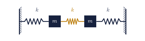
Fig. 93 The fixed-fixed mass-spring chain in its smallest nontrivial case \(N=2\): two equal masses \(m\) at their equilibrium spacing are joined to each other and to rigid walls by three identical springs of stiffness \(k\) (the central coupling spring shown in amber), giving the tridiagonal stiffness matrix of the equations of motion.

---

Setup

Data and instruments only: the unit mass and unit spring constant that fix the frequency scale, and an energy meter used as an integrator diagnostic. This notebook’s own machinery is not here — you build the stiffness matrix and the mode eigenproblem in Exercise 1, and the equations of motion in Exercise 5.

The Setup below holds this notebook’s data and instruments — nothing you are asked to build. It is collapsed so the building stays yours; expand it whenever you want the details.

Show code cell source

Hide code cell source

import numpy as np
from scipy.linalg import eigh
from scipy.integrate import solve_ivp
import matplotlib.pyplot as plt
from matplotlib.animation import FuncAnimation

from ecp import validate
from ecp.animate import show

# data: unit masses and unit spring constant unless noted, so frequencies come
# out in units of sqrt(k/m). The mass matrix is then the identity.
M_MASS = 1.0
K_SPRING = 1.0


# instrument: a diagnostic, not any exercise's lesson — the notebook uses the
# drift of this quadratic form to judge the integrator, and the meter itself is
# bookkeeping (a kinetic sum and the potential x·K·x/2 already written down in
# the theory section), not the craft this notebook teaches. It reads whatever
# stiffness matrix it is handed, including the ones your Exercise 1 `stiffness`
# builds.
def energy(s, K):
    """Total mechanical energy v·v/2 + x·K·x/2 (with M = I).

    Parameters
    ----------
    s : array_like
        State ``[x..., v...]``.
    K : numpy.ndarray
        Stiffness matrix.

    Returns
    -------
    float
        The total energy (an integrator check).
    """
    N = K.shape[0]
    x, v = s[:N], s[N:]
    return 0.5 * M_MASS * v @ v + 0.5 * x @ K @ x

Exercise 1 — Assemble the stiffness matrix and solve the eigenproblem

Everything starts from the matrix equation of motion Eq. 113. Because the system is linear, looking for single-frequency solutions collapses it to the generalised eigenvalue problem Eq. 114: the eigenvectors are the normal modes and the square roots of the eigenvalues are their frequencies. For a fixed–fixed chain of equal masses joined by equal springs \(k\) the stiffness matrix is tridiagonal — \(2k\) on the diagonal, \(-k\) on the two first off-diagonals, zero elsewhere. scipy.linalg.eigh solves the generalised problem directly, returning the eigenvalues in ascending order. For \(N=2\) the answer is known in closed form: the analytic pair Eq. 115.

1. Write stiffness(N, k=K_SPRING), returning the \(N \times N\) tridiagonal stiffness matrix of the fixed–fixed chain. Write this one yourself — the implementation is the lesson.

2. Write mode_frequencies(K, M=None): solve \(\mathsf K\,\mathbf v = \omega^2 \mathsf M\,\mathbf v\) with scipy.linalg.eigh(K, M) (identity mass matrix by default) and return the ascending mode frequencies — the square roots of the eigenvalues (numpy.sqrt), clipped at zero so rounding noise cannot produce a NaN — together with the matrix whose columns are the eigenvectors.

3. Build \(\mathsf K\) for \(N=2\) (two masses, fixed walls) and solve for its two mode frequencies. They should be the analytic pair of Eq. 115.

N=2 mode frequencies:  [1.         1.73205081]   (analytic: 1, √3 = 1.732051)

✓  N=2 mode frequencies are √(k/m), √(3k/m)   [max|Δ| = 0 (rtol=1e-10, atol=1e-09)]

True

Exercise 2 — Interpret the mode shapes

The eigenvectors carry the shape of each mode. For the two-mass system Eq. 115 predicts a low-frequency mode where the masses move together (in-phase, the spring between them barely stretches) and a high-frequency mode where they move oppositely (anti-phase, the middle spring does the most work). The sign pattern of the eigenvector components is what distinguishes them, and the two eigenvectors you need are the ones your Exercise 1 mode_frequencies already returned.

1. Identify the in-phase mode (lowest frequency, \(\omega_-\)) and the anti-phase mode (highest, \(\omega_+\)) by sorting on frequency (numpy.argsort).

2. Plot the two mode shapes as signed bars and confirm the in-phase mode has equal-sign components while the anti-phase mode has opposite signs.

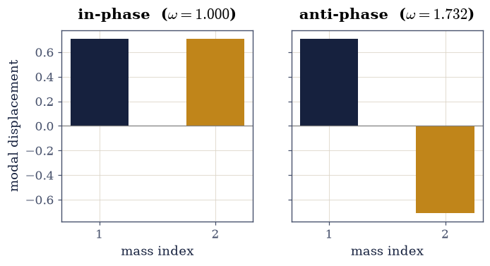
✓  ω₋ is in-phase, ω₊ is anti-phase   [in-phase product=+0.500, anti-phase product=-0.500]

True

Exercise 3 — Three masses: frequencies vs. the dispersion relation

The same machinery scales to any \(N\). For a fixed–fixed chain the spectrum is not arbitrary: it is fixed by the dispersion relation Eq. 116, which at \(N=3\) reads \(\omega_j = 2\sin(j\pi/8)\) for \(j=1,2,3\). The three-mass chain is the first case where the formula has an interior mode to get right.

1. Build the \(N=3\) chain with the stiffness you wrote in Exercise 1 and solve for its three frequencies with your mode_frequencies.

2. Compare them to \(\omega_j = 2\sin(j\pi/8)\), \(j=1,2,3\) from Eq. 116.

j=1   ω_num=0.765367   2 sin(jπ/8)=0.765367
j=2   ω_num=1.414214   2 sin(jπ/8)=1.414214
j=3   ω_num=1.847759   2 sin(jπ/8)=1.847759

✓  N=3 frequencies match 2 sin(jπ/8)   [max|Δ| = 1.11022e-16 (rtol=1e-10, atol=1e-09)]

True

Exercise 4 — The 1-D chain dispersion relation

Push \(N\) up and the discrete frequencies trace out the full dispersion curve of Eq. 116: nearly linear for the long-wavelength (small-\(j\)) modes, bending over to a flat band edge near \(j=N\). Plotting the numeric frequencies on top of the analytic sine is the clearest single picture of normal-mode theory.

1. Build the \(N=20\) chain and solve for all twenty frequencies, with the stiffness and mode_frequencies you wrote in Exercise 1.

2. Plot \(\omega_j\) against the mode index \(j\) and overlay the analytic dispersion curve of Eq. 116.

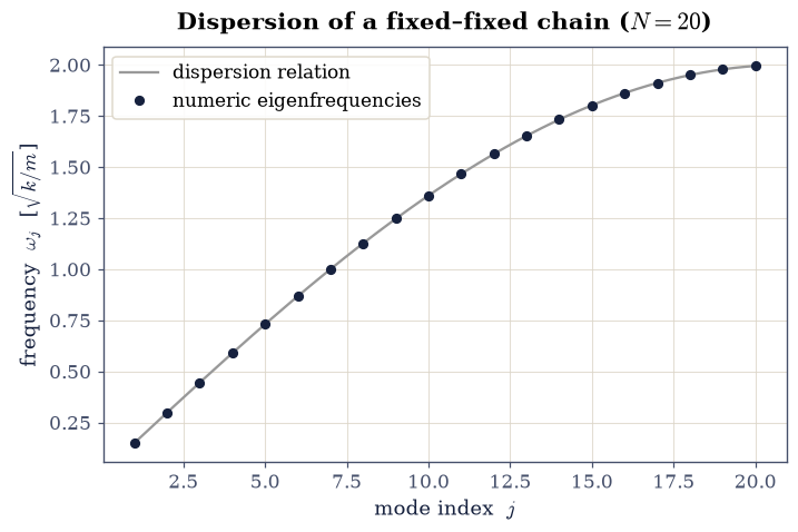
✓  chain spectrum matches the dispersion relation   [max|Δ| = 2.60902e-15 (rtol=1e-09, atol=1e-09)]

True

Exercise 5 — Time evolution conserves energy

Frequencies and shapes come from the static eigenproblem; to watch the system move we integrate Eq. 113 in time. A linear conservative system has no business gaining or losing energy, so the relative drift of the total energy is a direct check that the integrator is faithful: the same role conservation laws played for the orbit in §1.4. That energy is \(E=\tfrac12\mathbf v\cdot\mathbf v+\tfrac12\,\mathbf x^{\mathsf T}\mathsf K\mathbf x\), the Setup’s energy diagnostic. Integrating first needs Eq. 113 in the first-order form scipy.integrate.solve_ivp expects: a state \(\mathbf s = [\mathbf x, \mathbf v]\) stacking positions on velocities, whose derivative is \([\mathbf v, -\mathsf K\mathbf x/m]\).

1. Write rhs(t, s, K), that first-order form with \(\mathsf M = m\mathsf I\): split the state into its two halves and return the stacked derivative. Write this one yourself — the implementation is the lesson.

2. Pluck one mass of the \(N=2\) system (displace it, the other at rest) and integrate with scipy.integrate.solve_ivp (DOP853).

3. Confirm the total energy is conserved as the motion plays out.

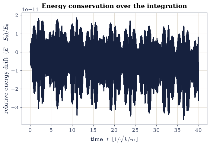
✓  total energy conserved (integrator check)   [max relative drift = 3.6673e-11 (limit 1e-06)]

True

Exercise 6 — A normal mode oscillates rigidly (worked animation)

Here is the defining property of a normal mode, made visible. Start the system exactly in one eigenvector and every mass oscillates at the single frequency \(\omega_j\) of Eq. 114, the spatial shape frozen: it only breathes up and down. No energy leaks into any other mode. This is the worked example for the two-animation rule; you build the second one in Exercise 7.

The animation shows the displacement profile of an \(N=8\) chain — assembled by the stiffness and mode_frequencies you wrote in Exercise 1 and advanced by your Exercise 5 rhs — initialised in one mode, scaling rigidly in time.

max amplitude leaked into other modes: 2.05e-15

Once Loop Reflect

Fig. 94 Animation of an \(N=8\) fixed-fixed chain initialised purely in its third-lowest normal mode (frequency \(\omega\)): every mass oscillates at the single frequency \(\omega\) so the spatial profile stays frozen and only its amplitude breathes, the defining property of a normal mode; the horizontal axis is the mass index.

✓  a pure normal mode does not excite the other modes   [got 2.05316e-15 vs expected 0 (rtol=1e-06, atol=1e-06)]

True

Exercise 7 — Beating (student-implemented animation)

Two identical oscillators tied to walls and coupled weakly to each other have two almost-equal mode frequencies. Start all the energy in one of them and the two modes (initially in phase) slowly drift apart and back, sloshing the energy entirely into the second oscillator and returning it, with the beat period Eq. 117. The first complete transfer happens at \(T_\mathrm{beat}/2\). Beating is the time-domain face of the two normal modes.

1. Build the two-oscillator system with wall springs \(k=1\) and a weak coupling spring \(\kappa = 0.05\) (its stiffness matrix is not the chain’s, so write it out directly), find its mode frequencies \(\omega_\pm\) with the mode_frequencies you wrote in Exercise 1, and integrate from \(x_1=1\), \(x_2=0\) (both at rest) over roughly one beat period with your Exercise 5 rhs and scipy.integrate.solve_ivp (DOP853).

2. Build the animation of the two masses sloshing energy back and forth: you have the trajectory x1(t), x2(t) below; assemble a FuncAnimation of the two masses on their springs, plt.close(fig), then display it with ecp.animate.show(anim).

3. Measure the first full-transfer time from the slow envelope of mass 2’s energy (a moving average via numpy.convolve) and compare it to \(T_\mathrm{beat}/2 = \pi/(\omega_+-\omega_-)\) from Eq. 117.

A ✗ on the final check is almost always about the measurement, not the physics: a raw argmax on mass 2’s fast-oscillating energy grabs a later revival. Smooth to the slow envelope (a moving average over about one fast period) before locating the first maximum.

ω_- = 1.00000,  ω_+ = 1.04881,  T_beat = 128.73
measured transfer time = 64.386,  T_beat/2 = 64.365

Once Loop Reflect

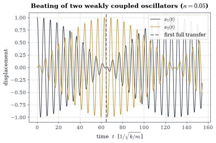
Fig. 95 Animation of two identical wall-anchored oscillators (\(k=1\)) joined by a weak coupling spring \(\kappa=0.05\), started with all energy in the left mass: the two masses (blue dots) slosh energy fully back and forth on the slow beat timescale \(T_\mathrm{beat}=2\pi/(\omega_+-\omega_-)\) set by the split between the two mode frequencies \(\omega_\pm\).

✓  energy fully transfers at T_beat/2   [got 64.3861 vs expected 64.3652 (rtol=0.005, atol=1e-09)]

True

Notebook summary

• The stiffness matrix and the eigenproblem \(K\mathbf v=\omega^2 m\mathbf v\) for the normal modes; the in-phase and out-of-phase mode shapes; and three masses checked against the monatomic-chain dispersion \(\omega=2\sqrt{k/m}\,|\sin(qa/2)|\).

• Time evolution conserving energy; a single normal mode oscillating rigidly at one frequency; and beating as the superposition of two near-degenerate modes.

Outlook

• Unequal masses or springs. Break the symmetry and watch the mode shapes distort: the heavier mass moves less in the high-frequency mode.

• The continuum limit. As \(N\to\infty\) the chain’s dispersion relation Eq. 116 becomes the wave equation’s \(\omega = c\,q\) for long wavelengths; compare the small-\(j\) slope to the sound speed.

• Free–free boundaries. Remove the walls and a zero-frequency mode appears, the uniform translation of the whole chain.

• Forced and damped. Drive one end and add damping; resonances appear exactly at the normal-mode frequencies found here.

References

[GPS02]

Herbert Goldstein, Charles P. Poole, and John L. Safko. Classical Mechanics. Pearson, 3 edition, 2002.

[Nol16a]

Wolfgang Nolting. Theoretical Physics 1: Classical Mechanics. Springer, 2016. Grundkurs Theoretische Physik 1.

[Nol16b]

Wolfgang Nolting. Theoretical Physics 2: Analytical Mechanics. Springer, 2016.

Take this notebook with you

Use the download button (↓) in the toolbar above to save this notebook and run it yourself. The published notebooks ship without worked solutions; if you would like the reference solutions — to teach from or to check your own work — get in touch: hello@ramador.me.