6.11 Bound States in One Dimension

Elementary Computational Physics

Volume VI — Quantum Mechanics Notebook 6.11

Trapping quantizes. A particle confined to a well has only a discrete ladder of allowed energies, and our grid solver finds them for any well shape. Symmetric wells sort their states by parity; deeper wells hold more of them; and two wells side by side reveal the most consequential structure of all — a pair of tunnelling-split levels that is, exactly, the two-state system we began the quantum story with.

Level · advanced   •   Est. · 160–195 min

Raymond Amador v1.4.0  ·  2026-07-31  ·  CC BY 4.0 (text) / MIT (code)

Notebook overview

In §6.10 we built an engine: hand it a potential on a grid and numpy.linalg.eigh returns the spectrum and the stationary states. This notebook uses that engine — we do not rebuild it — to do physics that pencil and paper struggle with, and it ends by reconnecting wave mechanics to the qubit that opened the volume.

The thread is confinement quantizes. A particle trapped in an attractive well has a discrete ladder of bound states (normalizable, with energy below the potential far away), and the grid method finds them for any well shape. We start with the finite square well, whose exact spectrum is set by a transcendental matching condition that has no closed-form solution — and watch the grid reproduce it without our doing any matching at all, a vivid demonstration of why the computational approach is liberating. A symmetric well brings in parity: because the Hamiltonian commutes with the reflection operator, every bound state is cleanly even or odd, and the parities alternate up the ladder — the first concrete case of a symmetry labelling states. We count how many states a well holds and find the one-dimensional rule that an attractive well always binds at least one.

Then the payoff. Put two wells side by side, and each single-well level splits into a near-degenerate doublet — a symmetric state just below, an antisymmetric one just above — separated by an energy that comes entirely from tunnelling through the central barrier and is exponentially sensitive to its width. The localized combinations are not energy eigenstates, so a particle placed in one well sloshes to the other and back. This doublet is not a curiosity: it is the ammonia molecule’s nitrogen inversion (the ammonia maser), and it is the physical origin of the qubit of §6.4. The abstract two-state system we began with turns out to be the most natural thing in the world — put a particle between two wells, and quantum mechanics hands you a qubit.

As in every Volume VI notebook, each exercise opens with a crystal-clear statement and enumerated parts, each naming the exact operation — the §6.10 finite-difference solver (numpy.linalg.eigh), scipy.optimize.brentq for the transcendental roots, and the parity diagnostic numpy.sum(psi*psi[::-1])*dx.

Method reuse. The hamiltonian/solve finite-difference eigensolver below is the one built and validated in §6.10 (the \((1,-2,1)/dx^2\) kinetic stencil plus \(\mathrm{diag}\,V\), diagonalized by numpy.linalg.eigh, eigenvectors normalized by \(\sqrt{dx}\)); we restate it for self-containment and then treat it purely as a tool — the new content here is the physics.

Conventions. \(\hbar=1\), \(m=1\). A symmetric grid on \([-L/2,L/2]\) (so the parity diagnostic psi[::-1] is exactly \(\psi(-x)\)), with the box large enough that bound-state wave functions decay before the edges. The finite well is \(V=-V_0\) for \(|x|<a\); the double well is two such wells centred at \(\pm x_c\). Numerical honesty: the tunnelling splitting falls exponentially with the barrier, and once it drops below the diagonalization floor (\(\sim10^{-13}\)) the computed doublet degeneracy is meaningless — we stay in the resolvable regime and say so (a §6.10 callback). See Griffiths (the finite well, parity, the double well); the Feynman Lectures Vol. III (the ammonia maser); and Notebooks §6.10 (the eigenmethod), §6.2 (parity commutes with \(H\)), §6.4 (the two-state system), §6.7 (tunnelling oscillation = two-level beating).

Theory in brief

Bound states and the discrete spectrum

A particle in an attractive well has bound states — normalizable eigenstates with energy below the potential at infinity,

(549)\[\hat H\psi_n=E_n\psi_n,\qquad E_n<0\ \text{(for a well vanishing at infinity)},\qquad \int|\psi_n|^2dx<\infty ,\]

forming a discrete spectrum (confinement quantizes), unlike the continuous spectrum of free states (§6.9). The §6.10 eigenmethod finds them: build \(H\) on a large box, diagonalize, keep the \(E<0\) levels.

The finite square well and the transcendental condition

For \(V=-V_0\) inside \(|x|<a\) and \(0\) outside, matching the interior oscillation (\(k=\sqrt{2m(E+V_0)}/ \hbar\)) to the exterior decay (\(\kappa=\sqrt{-2mE}/\hbar\)) at the walls gives the transcendental conditions

(550)\[k\tan(ka)=\kappa\ \text{(even)},\qquad -k\cot(ka)=\kappa\ \text{(odd)} ,\]

solvable only numerically (scipy.optimize.brentq). The grid method gives the same energies without doing the matching. Unlike the infinite well, the finite well has finitely many bound states, and the wave functions leak into the classically forbidden region (exponential tails — a tunnelling preview).

Parity

If \(V(-x)=V(x)\), then \(H\) commutes with the parity operator \(P\psi(x)=\psi(-x)\), so (§6.2) they share eigenstates: every bound state has definite parity,

(551)\[[H,P]=0\ \Longrightarrow\ \psi_n(-x)=\pm\psi_n(x),\qquad \text{ground state even, parities alternate} .\]

Parity is a conserved quantum number that halves the problem — the first concrete symmetry-labels-states example (the theme of complete sets of commuting observables, §6.6).

Bound-state counting

The number of bound states grows with depth and width; counting the crossings of the transcendental conditions above gives

(552)\[N_{\text{bound}}\approx\Big\lfloor\frac{2a}{\pi}\frac{\sqrt{2mV_0}}{\hbar}\Big\rfloor+1 ,\]

and a one-dimensional attractive well always binds at least one state, however shallow (unlike 3D). Each new state enters at threshold (\(E\to0\)) as the well deepens.

The double well and tunnelling doublets

Two wells separated by a barrier: each single-well level splits into a near-degenerate doublet, a symmetric (even) state just below and an antisymmetric (odd) state just above, split by \(\Delta E\),

(553)\[|L\rangle,|R\rangle=\tfrac{1}{\sqrt2}(|\text{sym}\rangle\pm|\text{antisym}\rangle),\qquad T=\frac{2\pi\hbar}{\Delta E},\qquad \Delta E\ \text{exponentially small in the barrier} .\]

The localized \(|L\rangle,|R\rangle\) are not energy eigenstates, so a particle in one well tunnels to the other with period \(T=2\pi\hbar/\Delta E\) (the §6.7 beating of two energy eigenstates). This is the ammonia molecule and the physical origin of the qubit of §6.4: the symmetric/antisymmetric doublet is the qubit’s \(|0\rangle/|1\rangle\), the tunnelling splitting its energy gap.

Setup

The data are the series palette, the conventions \(\hbar=1\) and \(m=1\), and the symmetric grid on \([-L/2,L/2]\) that makes the reversed array psi[::-1] exactly \(\psi(-x)\) — the fixed stage every well below is placed on. The instruments are the §6.10 eigensolver, restated here for self-containment and used purely as a tool — hamiltonian and solve, both of which you built there, so here they are earned equipment. The rest are one-liners the text spells out as it uses them: the parity diagnostic \(\int\psi(x)\psi(-x)\,dx\), the count of negative eigenvalues, and the localized combinations \((|\text{sym}\rangle\pm|\text{antisym}\rangle)/\sqrt2\) transcribed straight from Eq. 553. The one piece of machinery this notebook asks you to construct is not here: you write transcendental_roots in Exercise 2.

The Setup below holds this notebook’s data and instruments — nothing you are asked to build. It is collapsed so the building stays yours; expand it whenever you want the details.

Show code cell source

Hide code cell source

import matplotlib.pyplot as plt
import numpy as np
from matplotlib.animation import FuncAnimation
from scipy.optimize import brentq

from ecp import draw, validate
from ecp.animate import show

# data: the series palette
ACCENT, INK, SOFT = draw.ACCENT, draw.INK, draw.SOFT
RED = "#c1121f"

# data: conventions
HBAR = 1.0  # ℏ = 1
MASS = 1.0  # m = 1

# data: a symmetric grid on [−L/2, L/2] so that psi[::-1] is exactly ψ(−x) (the parity diagnostic).
L_BOX = 20.0
N_GRID = 1400
X = np.linspace(-L_BOX / 2, L_BOX / 2, N_GRID)
DX = X[1] - X[0]


# built from scratch in §6.10; restated here as an instrument.
def hamiltonian(x, V):
    """The §6.10 finite-difference Hamiltonian: $-(\\hbar^2/2m)(1,-2,1)/dx^2$ stencil plus $\\mathrm{diag}\\,V$.

    Restated from §6.10 for self-containment (assembled with ``numpy.diag``); a real symmetric matrix.
    """
    n = len(x)
    dx = x[1] - x[0]
    lap = (
        np.diag(-2 * np.ones(n))
        + np.diag(np.ones(n - 1), 1)
        + np.diag(np.ones(n - 1), -1)
    ) / dx**2
    return -(HBAR**2 / (2 * MASS)) * lap + np.diag(V)


# built from scratch in §6.10; restated here as an instrument.
def solve(x, V):
    """Diagonalize: energies and normalized stationary states (the §6.10 eigenmethod, reused) {eq}`eq-bound`.

    ``numpy.linalg.eigh`` returns sorted real eigenvalues and orthonormal eigenvectors; columns are
    divided by $\\sqrt{dx}$ so $\\int|\\psi_n|^2dx=1$. We *use* this as a tool here; it was built and
    validated in §6.10.
    """
    energies, states = np.linalg.eigh(hamiltonian(x, V))
    return energies, states / np.sqrt(x[1] - x[0])


# instrument: the parity reading, one inner product against the reversed array. The expression is
# spelled out in the overview and in Exercise 3 itself; what Exercise 3 teaches is what the numbers
# say — definite ±1, even ground state, strict alternation — not how to type the sum.
def parity(psi, dx):
    """The parity diagnostic $\\int\\psi(x)\\psi(-x)\\,dx$ {eq}`eq-parity`.

    On a grid symmetric about the origin, $\\psi(-x)$ is the reversed array ``psi[::-1]``, so this is
    ``numpy.sum(psi*psi[::-1])*dx``. For a normalized definite-parity state it returns $+1$ (even) or
    $-1$ (odd).
    """
    return np.sum(psi * psi[::-1]) * dx


# instrument: reading a count off the spectrum, ``numpy.sum(energies < 0)``. Exercise 4 teaches how
# that count grows with the depth of the well, which is physics; the tally itself is not.
def count_bound(energies):
    """The number of bound states — the count of negative eigenvalues {eq}`eq-counting`."""
    return int(np.sum(energies < 0))


# data: the two localized superpositions exactly as the double-well equation displays them,
# (|sym⟩ ± |antisym⟩)/√2 — a given combination with nothing to construct beyond the two signs.
def localized_states(sym, antisym):
    """The localized combinations $|L\\rangle,|R\\rangle=(|\\text{sym}\\rangle\\pm|\\text{antisym}\\rangle)/\\sqrt2$ {eq}`eq-double-well`.

    Two equal superpositions of the symmetric and antisymmetric doublet members; each is concentrated in
    one well. They are *not* energy eigenstates, so they tunnel.
    """
    return (sym + antisym) / np.sqrt(2), (sym - antisym) / np.sqrt(2)

Exercise 1 — The finite square well: spectrum and leaking wave functions

Solve a finite square well \(V=-V_0\) for \(|x|<a\) (and \(0\) outside) and find its bound states. Report the bound energies and observe that the eigenfunctions leak into the classically forbidden region with exponential tails Eq. 549, Eq. 550.

1. Build \(V=-V_0\) for \(|x|<a\) on the large box X with numpy.where.

2. Solve with the §6.10 solve helper (numpy.linalg.eigh) and keep the \(E<0\) eigenvalues — the bound states.

3. Report how many there are and their energies (finitely many, unlike the infinite well).

4. Plot the eigenfunctions and note the exponential tails extending past \(|x|=a\) into the forbidden region — the wave function penetrates the wall, a tunnelling preview.

finite well V0=18.0, a=1.0: 4 bound states (E<0)
  bound energies: [-17.0972 -14.4176 -10.0691  -4.3655]
  ground-state probability in the forbidden region |x|>a: 0.007  (leaks past the wall)

Validation 1

✓  a finite well binds a discrete, finite set of states (E<0) whose wave functions leak into the classically forbidden region

True

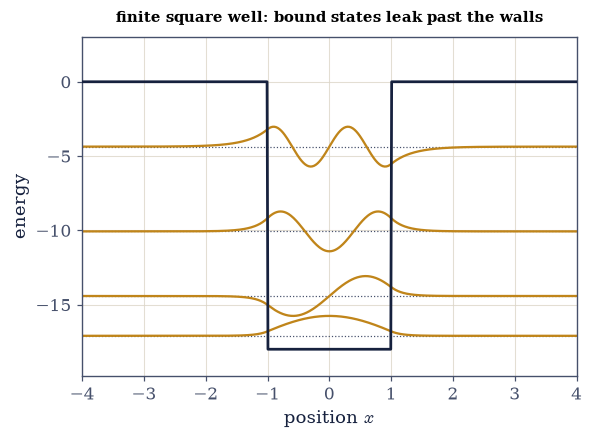
Fig. 535 The finite square well. The well of depth \(V_0\) and half-width \(a\) (ink) with its bound levels (dotted) and stationary states (amber) drawn at their energies. Unlike the infinite well, there are only finitely many bound states, and each wave function does not stop at the wall: it leaks past \(|x|=a\) into the classically forbidden region with an exponential tail, because a quantum particle has a nonzero amplitude to be where a classical one could never go. That penetration is the seed of tunnelling — and, two wells over, of the qubit. The parities alternate, even–odd–even–odd, up the ladder.

Exercise 2 — The transcendental condition, checked against the grid

The finite well’s exact spectrum comes from matching the interior oscillation to the exterior decay at the walls, which gives the conditions \(k\tan(ka)=\kappa\) (even) and \(-k\cot(ka)=\kappa\) (odd), with \(k=\sqrt{2m(E+V_0)}/\hbar\) and \(\kappa=\sqrt{-2mE}/\hbar\) Eq. 550. They are transcendental: there is no closed form for the energies in \((-V_0,0)\) that satisfy them, only a numerical search. The search is cleanest in the dimensionless variable \(u=ka\), where the two conditions read \(u\tan u=\sqrt{R^2-u^2}\) and \(-u\cot u=\sqrt{R^2-u^2}\) with \(R=\sqrt{2mV_0a^2}/\hbar\) the well-strength radius that packages depth, width and mass into one number. In that variable each branch lives between consecutive poles of \(\tan\) or \(\cot\), so a bracket taken on \((n\pi,(n+\tfrac12)\pi)\) for the even branches and on \(((n+\tfrac12)\pi,(n+1)\pi)\) for the odd ones, each clipped at \(R\), encloses at most one root and never straddles a divergence. That bracketing is the whole trick: scipy.optimize.brentq needs a sign change across the bracket, and a pole would hand it a false one. Roots come back as energies through \(E=(\hbar^2/2m)(u/a)^2-V_0\). Expect the deepest levels to match the grid to \(\sim10^{-3}\) and the shallowest — most diffuse, and sitting at the well’s discontinuous edge — to \(\sim10^{-2}\), the resolution caveat of §6.10.

1. Write transcendental_roots(V0, a), returning the sorted bound energies of the finite well by solving both branches of the matching condition with scipy.optimize.brentq, bracket by bracket in \(u\). Write this one yourself — the implementation is the lesson.

2. Compare its roots to the grid spectrum of Exercise 1.

3. Confirm the two agree, to the tolerances above. The grid method is liberating: the same answer, and no transcendental algebra.

transcendental roots (brentq): [-17.0958 -14.4121 -10.0566  -4.3447]
grid eigenvalues:              [-17.0972 -14.4176 -10.0691  -4.3655]
agreement (same count 4=4): max|Δ| = 2.1e-02
  (deepest levels agree to ~1e-3; the shallowest, most diffuse, to ~1e-2 — the §6.10 resolution caveat)

Validation 2

✓  the grid spectrum matches the finite well's transcendental matching condition (without our doing the matching)   [max|Δ| = 0.0208405 (rtol=1e-06, atol=0.05)]

True

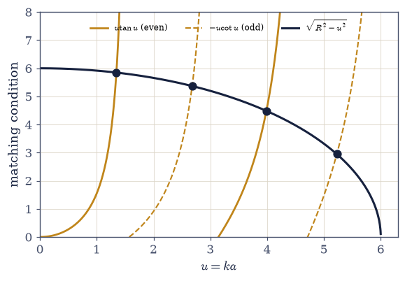
Fig. 536 The transcendental condition, graphically. The finite well’s even bound states sit where \(u\tan u\) (amber) meets the quarter-circle \(\sqrt{R^2-u^2}\) (ink), and the odd states where \(-u\cot u\) (dashed) meets it, with \(u=ka\) and \(R=\sqrt{2mV_0a^2}/\hbar\) the well-strength radius (grey). The crossings (dots) are the allowed energies — there is no closed form for them, only this graphical/numerical intersection, which scipy.optimize.brentq finds branch by branch. The grid eigensolver of §6.10 lands on exactly the same energies without any of this matching: it simply diagonalizes the matrix. That is the liberation of the computational method.

Exercise 3 — Parity

Show that the bound states of the symmetric finite well have definite parity, even or odd, with the ground state even and the parities alternating up the ladder Eq. 551.

1. Confirm the potential is symmetric, \(V(-x)=V(x)\) (the grid is symmetric, so numpy.allclose(V, V[::-1])), which makes \([H,P]=0\).

2. For each bound state compute the parity diagnostic \(\int\psi(x)\psi(-x)\,dx\) with the parity helper (numpy.sum(psi*psi[::-1])*dx).

3. Confirm each value is \(+1\) (even) or \(-1\) (odd).

4. Observe the ground state is even and the parities alternate \(+,-,+,-,\dots\). Parity is a conserved quantum number handed over by a symmetry (§6.2 — \(P\) and \(H\) share eigenstates), and it halves the problem.

V(−x)=V(x) (symmetric, so [H,P]=0): True
parities of the bound states: [ 1. -1.  1. -1.]
  → ground state even (+1), alternating: ['even', 'odd', 'even', 'odd']

Validation 3

✓  a symmetric well gives definite-parity eigenstates (±1), even ground state, parities alternating up the ladder

True

Exercise 4 — Bound-state counting

Determine how the number of bound states depends on the well depth \(V_0\), compare to the estimate \(\lfloor(2a/\pi)\sqrt{2mV_0}/\hbar\rfloor+1\), and confirm the one-dimensional rule that even a shallow well binds at least one state Eq. 552.

1. Solve the well for a range of depths \(V_0\) (the solve helper at each).

2. Count the \(E<0\) states with count_bound.

3. Compare to the estimate \(\lfloor(2a/\pi)\sqrt{2mV_0}/\hbar \rfloor+1\).

4. Confirm the count rises in steps as \(V_0\) grows (a new state enters at threshold), and that even the shallowest well has \(\ge1\) bound state. Deeper and wider wells hold more; a 1-D attractive well always binds.

V0     bound-state count    estimate ⌊(2a/π)√(2mV0)⌋+1
  0.5        1                  1
  2.0        2                  2
  5.0        2                  3
 10.0        3                  3
 20.0        5                  5
 40.0        6                  6
 70.0        8                  8

shallowest well (V0=0.5) still binds 1 state — a 1-D attractive well always binds ≥ 1

Validation 4

✓  the bound-state count grows with depth (matching the threshold estimate) and is ≥1 even for a shallow well

True

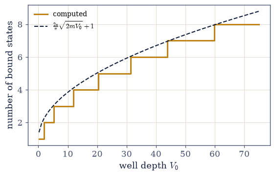
Fig. 537 Deeper wells hold more states. The number of bound states of the finite well as its depth \(V_0\) increases (amber staircase), tracking the estimate \(\lfloor(2a/\pi)\sqrt{2mV_0}/\hbar\rfloor+1\) (ink). Each step up marks a new bound state appearing at threshold (\(E\to0\)) as the well deepens enough to hold it. The staircase never drops to zero: in one dimension, any attractive well — however shallow — binds at least one state, a special feature of 1-D (a shallow 3-D well may bind none). Counting bound states is thus reading off how many rungs the confinement ladder has.

Exercise 5 — The double well and tunnelling doublets

Solve a symmetric double well — two wells separated by a barrier — and analyze its lowest doublet: confirm the two lowest states are a near-degenerate pair, a symmetric (even) state just below an antisymmetric (odd) one, and that their \(\pm\) combinations localize in the two wells Eq. 553.

1. Build two wells of depth \(V_0\) and half-width \(a\) centred at \(\pm x_c\) with numpy.where.

2. Solve with the solve helper.

3. Identify the lowest two states as a doublet: confirm their parities (even below, odd above, via the parity helper) and measure the splitting \(\Delta E=E_1-E_0\) — tiny compared with the gap to the next level.

4. Form the localized combinations \(|L\rangle,|R\rangle=(|\text{sym}\rangle\pm|\text{antisym}\rangle)/\sqrt2\) with localized_states and show each is concentrated in one well. Tunnelling splits each single-well level into a doublet.

double well (V0=8.0, a=0.8, x_c=1.3):
  doublet: E0 = -6.90716 (parity +1.00), E1 = -6.88383 (parity -1.00)
  splitting ΔE = 2.3331e-02   (gap to next level = 3.033 — the doublet is isolated)
  localized: |L⟩ probability in x<0 = 1.000;  |R⟩ in x<0 = 0.000

Validation 5

✓  tunnelling splits the level into a symmetric/antisymmetric doublet, whose ± combinations localize in the two wells

True

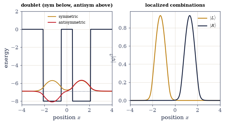
Fig. 538 The tunnelling doublet. Left: the double well (ink) and the lowest doublet — a symmetric (even) state just below an antisymmetric (odd) state, split by a tiny \(\Delta E\) that comes entirely from tunnelling through the central barrier. Right: their equal combinations \((|\text{sym}\rangle\pm|\text{antisym}\rangle)/\sqrt2\) are localized, one in each well. These localized states are not energy eigenstates, so a particle prepared in one well does not stay — it tunnels to the other and back. This doublet is a two-state system: the symmetric and antisymmetric states are the qubit’s \(|0\rangle\) and \(|1\rangle\), and \(\Delta E\) is its energy gap.

Exercise 6 — Tunnelling oscillation and the qubit connection

Show that a particle localized in one well tunnels to the other and back with period \(T=2\pi\hbar/\Delta E\), and identify this two-state system with the qubit of §6.4 Eq. 553.

1. Start in \(|L\rangle\) (not an energy eigenstate, but \((|\text{sym}\rangle+|\text{ antisym}\rangle)/\sqrt2\)).

2. Evolve it (§6.7): each doublet member carries its phase \(e^{-iE_nt/ \hbar}\), so \(|\psi(t)\rangle=(e^{-iE_0t}|\text{sym}\rangle+e^{-iE_1t}|\text{antisym}\rangle)/\sqrt2\).

3. Compute the probability in the right well versus time and confirm it oscillates with period \(T=2\pi\hbar/\Delta E\) (the two energies beat — §6.7).

4. Identify the symmetric/antisymmetric doublet as the qubit’s \(|0\rangle/|1\rangle\) and \(\Delta E\) as its gap: this is the ammonia molecule’s inversion and the physical origin of the §6.4 qubit. The abstract two-state system is derived here from a potential, not postulated.

tunnelling period T = 2πℏ/ΔE = 269.3
right-well probability: starts 0.000, reaches 0.999 at half a period, returns to 0.000
→ the symmetric/antisymmetric doublet IS the qubit's |0⟩/|1⟩; ΔE is its gap (the ammonia maser, the §6.4 two-state system).

Validation 6

✓  a particle localized in one well tunnels fully to the other and back with period 2πℏ/ΔE — the tunnelling doublet is a two-state system   [max|Δ| = 0.000549608 (rtol=1e-06, atol=0.05)]

True

Once Loop Reflect

Fig. 539 Tunnelling, animated — the ammonia molecule and the qubit. A particle prepared in the left well (not an energy eigenstate, but the superposition \((|\text{sym}\rangle+|\text{antisym}\rangle)/\sqrt2\)) does not stay: its probability density \(|\psi(x,t)|^2\) (amber) sloshes through the barrier into the right well and back, with period \(T=2\pi\hbar/\Delta E\). This is the §6.7 beating of two energy eigenstates, made spatial — and it is exactly the nitrogen atom of an ammonia molecule tunnelling through the plane of its hydrogens, the oscillation that runs the ammonia maser. The two-state system we postulated in §6.4 is here derived: two wells, a barrier, and a particle that cannot decide which side it is on.

Exercise 7 — Splitting versus barrier, and where the numerics would run out (student)

Study how the doublet splitting \(\Delta E\) depends on the barrier width (the well separation), and mark the floor below which the computation would stop being trustworthy Eq. 553.

1. Compute \(\Delta E\) for a series of separations \(x_c\) (wider \(x_c\) = wider barrier), each via the solve helper.

2. Plot \(\Delta E\) on a log scale against \(x_c\) and observe the exponential decrease (a straight line on the log plot — tunnelling is exponentially sensitive to the barrier).

3. Mark the diagonalization floor (\(\sim10^{-13}\)) below which the computed doublet degeneracy would become meaningless, and confirm the scan stays above it — in the resolvable regime.

4. State the lesson: the exponential trend is physics; the floor is where the numerics would run out, and stopping above it is honest computation (a §6.10 callback). Tunnelling — and the limit of our precision — are both exponential in the barrier.

separation x_c    splitting ΔE
   0.9            4.654e-01
   1.2            4.906e-02
   1.5            5.278e-03
   1.8            5.678e-04
   2.1            6.108e-05
   2.4            6.572e-06
   2.7            7.070e-07
   3.0            7.606e-08
   3.3            8.183e-09
   3.6            8.803e-10
   3.9            9.471e-11
   4.2            1.019e-11  ← smallest, still above the ~1e-13 floor

exponential decay: ΔE ∝ exp(-7.43·x_c) where resolvable — roughly 1693× smaller per unit of separation

Validation 7

✓  the tunnelling splitting decreases exponentially with barrier width, staying above the numerical floor (~1e-13) below which the numerics would run out

True

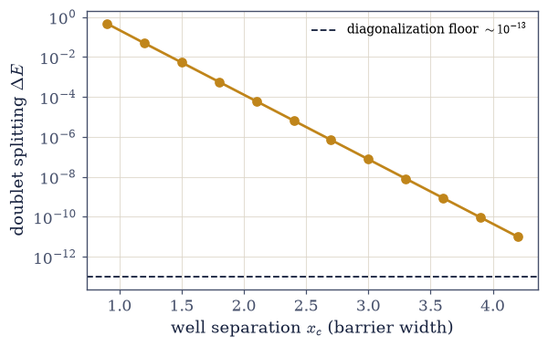
Fig. 540 Tunnelling is exponentially sensitive to the barrier. The doublet splitting \(\Delta E\) against the well separation \(x_c\) (wider \(x_c\) = thicker barrier), on a log scale (amber). It falls along a straight line — \(\Delta E\) shrinks roughly an order of magnitude for every small increase in separation, the exponential signature of tunnelling through a barrier. The dashed line marks the diagonalization floor (\(\sim10^{-13}\)): below it the two doublet members would be numerically degenerate and numpy.linalg.eigh could no longer resolve them, so the computed splitting would be meaningless (a §6.10 callback). This scan stays comfortably above that floor — the whole curve is physics, and stopping before the arithmetic runs out is the discipline of computational physics.

Exercise 8 — Confinement, symmetry, and the birth of the two-state system (synthesis)

Trapping a particle quantizes its energy into a discrete ladder; a symmetric well sorts that ladder by parity; deeper wells hold more rungs, and in one dimension even the shallowest well holds at least one. The finite well showed the spectrum is set by a transcendental condition the grid solves for free, and that bound states leak past their walls. And when two wells sit side by side, that leakage becomes tunnelling: each rung splits into a doublet whose two members beat against each other, a particle sloshing from well to well with period \(2\pi\hbar/\Delta E\).

There is no new computation here; the connection is the result. That doublet is not a curiosity — it is the ammonia molecule’s inversion, and it is the qubit we began the quantum story with in §6.4, now derived from a potential rather than postulated. We opened this volume with an abstract two-state system and called it the simplest quantum object; here it turns out to be the most natural one, handed to us by quantum mechanics the moment we place a particle between two wells. The next notebook (§6.12) solves the single most important bound-state problem of all — the harmonic oscillator, the universal description of any system near a minimum — both by diagonalizing on the grid and by the elegant algebra of ladder operators.

Notebook summary

The §6.10 eigenmethod applied to bound-state physics — and the qubit, derived.

• Bound states Eq. 549: confinement gives a discrete ladder of normalizable \(E<0\) states; the §6.10 solver finds them for any well.

• The finite well Eq. 550: finitely many states, set by a transcendental condition (scipy.optimize.brentq, branch by branch) that the grid reproduces without matching; wave functions leak past the walls.

• Parity Eq. 551: a symmetric well gives definite-parity states (\(\int\psi(x)\psi(-x)dx= \pm1\)), even ground state, alternating — a symmetry labelling states (\([H,P]=0\), §6.2).

• Counting Eq. 552: the number of states grows with depth (\(\approx\lfloor(2a/\pi) \sqrt{2mV_0}/\hbar\rfloor+1\)); a 1-D well always binds \(\ge1\).

• The double well Eq. 553: tunnelling splits each level into a symmetric/antisymmetric doublet; the localized \((|\text{sym}\rangle\pm|\text{antisym}\rangle)/\sqrt2\) tunnel with period \(2\pi\hbar/\Delta E\); \(\Delta E\) is exponentially small in the barrier (until the \(\sim10^{-13}\) numerical floor).

This doublet is the ammonia molecule and the physical origin of the §6.4 qubit: the two-state system we postulated, now derived from a potential.

Outlook

• The harmonic oscillator (§6.12): ladder operators and the analytic solution, checked against the grid; coherent states.

• Scattering and tunnelling through barriers (§6.13): transmission, resonances, wave-packet dynamics.

• Identical particles (§6.20): the same symmetric/antisymmetric structure in a new role.

• Molecular physics: tunnelling, inversion, and the ammonia maser (a horizon).

• Cross-reference §6.10 (the eigenmethod), §6.2 (parity / commuting operators), §6.4 (the two-state system), §6.7 (tunnelling oscillation = two-level beating), and forward to §6.12, §6.13, §6.20.

Take this notebook with you

Use the download button (↓) in the toolbar above to save this notebook and run it yourself. The published notebooks ship without worked solutions; if you would like the reference solutions — to teach from or to check your own work — get in touch: hello@ramador.me.