7.15 Einstein’s A and B Coefficients: Thermodynamics Predicts the Laser

Elementary Computational Physics

Volume VII — Quantum Statistical Mechanics Notebook 7.15

In 1917 Einstein wrote down three rates for how atoms exchange light — one of them a process nobody had ever seen — and showed that Planck's law leaves no choice: without stimulated emission, equilibrium light comes out wrong in the classical limit itself. We run the argument forwards and backwards, map where spontaneous and stimulated emission each rule, prove that two levels can never lase while four levels barely try, keep this volume's negative-temperature promise in a ruby rod, and watch a minimal laser snap through threshold.

Level · advanced   •   Est. · 190–230 min

Raymond Amador v1.4.0  ·  2026-07-31  ·  CC BY 4.0 (text) / MIT (code)

Notebook overview

§7.14 built the gas; this notebook asks how matter talks to it, and answers with one of the most beautiful arguments in physics: Einstein 1917, run the way it was written: thermodynamics in reverse. Take two-level atoms bathed in radiation and write three rates whose coefficients nobody in 1917 could derive: absorption \(N_1B_{12}u\), stimulated emission \(N_2B_{21}u\), and spontaneous emission \(N_2A\). Demand that the steady state reproduce Planck’s law at every temperature (the law of §7.14 is not negotiable) and the demand does the deriving: \(g_1B_{12} = g_2B_{21}\) (absorption and stimulated emission are one matrix element read in opposite directions) and \(A/B_{21} = \hbar\omega^3/\pi^2c^3\). The teaching move is the counterfactual, with teeth: switch stimulated emission off and the same steady state produces Wien’s exponential, which fails the classical Rayleigh–Jeans limit by a factor of twenty at \(x = 0.05\) (measured below: \(u\cdot x = 0.048\) against Planck’s 0.975). The classical limit itself testifies that emission must be enhanced by the light already present. Einstein predicted a process from thermodynamic consistency in 1917; Maiman built its consequence in 1960.

The forced ratio has a meaning that organizes the whole movement: per atom, stimulated/spontaneous \(= \bar n(\omega, T)\) exactly, so total emission scales as \(\bar n + 1\): the boson enhancement, one family with the bunching variance \(n(1+n)\) of §7.7 and Volume VI’s ladder element \(\sqrt{n+1}\), with QED’s reading of the \(+1\) as stimulation by the vacuum named as the horizon this argument leapfrogged. We quantify the landscape: \(\bar n = 1\) along \(\hbar\omega = k_BT\ln 2\) (4.33 THz at 300 K), sodium’s D line at room temperature sits at \(\bar n \sim 10^{-36}\) (hot matter glows: the optical world belongs to spontaneous emission), while the 21-cm line sits at \(\bar n \approx 4400\) (the radio universe is stimulated, which is why masers preceded lasers). The computational centerpiece is inversion by steady-state rate equations: the two-level no-go (\(N_2/N_1\) saturates at 0.9999 under a \(10^4\times\) drive and never crosses one), ruby’s three-level scheme inverting only when the pump beats \(A\), at which point more than half of all atoms are airborne, and the four-level scheme inverting at any pump whatsoever (\(P/A = 0.01\) verified). The negative-temperature promise of §7.4 is kept here: an inverted pair is a Boltzmann population at \(T < 0\) (\(N_2/N_1 = 1.5\) reads \(-51\,000\) K at the ruby line), and the \(\beta\)-axis picture explains the upside-down ordering. A data exercise decomposes the \(\omega^3\) tyranny honestly, sodium’s 16 ns against the 21-cm line’s eleven million years: 22.3 orders of magnitude, of which the forced \(\omega^3\) law supplies 16.7 and magnetic-dipole forbiddenness the remaining 5.7. The stretch assembles a minimal single-mode laser and watches it snap through threshold: photon number rising linearly above \(P_{\text{th}}\) while the inversion clamps: a nonequilibrium phase transition, named.

Conventions (this notebook). For the structural argument the spectral density \(u\) is measured in units of \(A/B_{21}\) and frequencies in \(x = \hbar\omega/k_BT\); SI units return for the data (cited transition rates: \(A(\text{Na D}) = 6.16\times10^7\) s⁻¹, \(A(\text{21 cm}) = 2.85\times10^{-15}\) s⁻¹ — NIST ASD and Wild 1952 lineage, cited not tuned). Degeneracy factors are kept symbolic through the forced relations and set to \(g_1 = g_2 = 1\) afterwards, where stated. Every \(\bar n\) uses numpy.expm1; steady states come from flow balance with the conservation row checked explicitly (and numpy.linalg.solve as the general cross-check); the laser steady state uses scipy.optimize.brentq with a deliberately asymmetric bracket (stated where used). Level diagrams precede algebra.

How to read the checks. Each exercise closes with a validate call against an independent fact: the steady-state spectrum solved numerically (brentq on the rate balance) against the analytic Planck form; the counterfactual’s factor-20 failure at small \(x\); the landscape numbers; the two-level saturation ceiling; the closed-form flow balances against the general linear solve at \(10^{-10}\); the negative-temperature ladder; the \(\omega^3\) decomposition against cited data; the threshold kink and clamp. A ✓ is strong evidence; a ✗ is a prompt to locate the discrepancy.

Scope. The QED derivation of \(A\) (vacuum fluctuations; the \(+1\) at \(n = 0\)), Rabi oscillations and saturation spectroscopy, and astrophysical masers are named horizons. See Einstein 1917 (“Zur Quantentheorie der Strahlung”); Maiman 1960; Siegman, Lasers; Loudon, The Quantum Theory of Light. Cross-reference §7.14 (the gas; Planck non-negotiable), §7.4 (the Boltzmann ratio, and the negative-temperature seed planted there), §7.7 (the \((n+1)\) family), §6.24 (the golden rule for \(B\), invoked), §7.5 (the oscillator per mode), and forward to §7.16 (phonons) and §7.17 (BEC, where bosonic amplification happens to matter waves).

Theory in brief

The three rates and the steady state

Einstein’s 1917 postulates for a two-level atom (\(E_2 - E_1 = \hbar\omega_0\), degeneracies \(g_1, g_2\)) in radiation of spectral density \(u(\omega_0)\):

(771)\[\text{absorption: } N_1B_{12}u, \qquad \text{stimulated emission: } N_2B_{21}u, \qquad \text{spontaneous emission: } N_2A .\]

The honesty note first: in 1917 none of these coefficients was derivable: \(B\) would wait for the golden rule (§6.24), \(A\) for quantum electrodynamics. Einstein simply postulated the forms and let equilibrium do the rest. In the steady state, up-flow equals down-flow, \(N_1B_{12}u = N_2(B_{21}u + A)\), and the populations obey the Boltzmann ratio of §7.4 \(N_2/N_1 = (g_2/g_1)e^{-\hbar\omega_0/k_BT}\). Solving for the spectral density the atoms would enforce:

\[u \;=\; \frac{A/B_{21}}{\dfrac{g_1B_{12}}{g_2B_{21}}\,e^{\hbar\omega_0/k_BT} - 1} .\]

Planck forces the relations

This must equal Planck’s law — for every temperature, since the atoms’ level spacing knows nothing of the walls’. Matching the \(T \to \infty\) behaviour and the overall form:

(772)\[g_1B_{12} = g_2B_{21}, \qquad \frac{A}{B_{21}} = \frac{\hbar\omega^3}{\pi^2c^3} .\]

The first says absorption and stimulated emission are the same matrix element read in opposite directions (the golden-rule symmetry of §6.24, invoked); the second prices spontaneous emission in terms of stimulated. The counterfactual gives the argument teeth: set \(B_{21} = 0\) and the same steady state yields \(u \propto e^{-\hbar\omega/k_BT}\), Wien’s law, which fails the classical Rayleigh–Jeans limit by a factor of 20 at \(x = 0.05\) (verified: \(u\cdot x = 0.048\) against 0.975). The classical limit itself demands that emission be enhanced by the light already present. History in two sentences: Einstein predicted stimulated emission from thermodynamic consistency in 1917; Maiman switched on the first laser in 1960. The division of labor: \(B\) is computable from §6.24 (invoked, one line); \(A\) then follows for free from the ratio: equilibrium constraining microphysics that 1917 mechanics could not reach, with the QED derivation (vacuum fluctuations; the \(+1\) surviving at \(n = 0\)) named as the horizon.

Stimulated/spontaneous = n̄: the landscape

Divide the two emission rates, using both forced relations and Planck’s \(u\):

(773)\[\frac{\text{stimulated}}{\text{spontaneous}} = \frac{B_{21}u}{A} = \frac{1}{e^{\hbar\omega/k_BT} - 1} = \bar n(\omega, T), \qquad \text{total emission} \propto \bar n + 1 .\]

The family reunion, in one paragraph: this \((\bar n + 1)\) is the boson bunching of §7.7 (the variance \(\langle\Delta n^2\rangle = \bar n(1 + \bar n)\) grew from the same enhancement), Volume VI’s ladder element \(a^\dagger|n\rangle = \sqrt{n+1}\,|n+1\rangle\) squared, and — in QED’s reading — stimulation by the vacuum: spontaneous emission is the \(+1\) that survives when \(n = 0\). The crossover \(\bar n = 1\) sits at \(\hbar\omega = k_BT\ln 2\), i.e. 4.33 THz at 300 K. Above it the world glows (sodium D at 300 K: \(\bar n \sim 4\times10^{-36}\); spontaneous emission owns the optical world); near it sits the CO₂ laser line (0.011); far below it the 21-cm line (\(\bar n \approx 4400\)) lives in a stimulated radio universe, which is why the maser preceded the laser, and why OH, H₂O, and SiO masers glow unpumped in comet comae and stellar envelopes.

The two-level no-go

Drive the lasing transition itself as hard as physics allows:

(774)\[\frac{N_2}{N_1} = \frac{B u}{A + B u} \;<\; 1 \quad\text{for every finite drive} \qquad (g_1 = g_2) ,\]

saturating at 0.9999 under a \(10^4\times\) drive (verified) and never inverting: absorption and stimulated emission ride the same matrix element, so the harder one pumps, the harder the medium de-excites. The forced relation returns as an engineering verdict. Equalization is the ceiling; this universal flattening is saturation (the Rabi physics of §6.24 is one breath away, named not developed).

Three and four levels: the pumping economics

The no-go forbids inverting the pair one drives, so every working laser adds levels: pump one transition, lase another, and let the steady state of the full rate equations decide whether inversion appears (Siegman’s Lasers develops the machinery at textbook length):

(775)\[\text{3-level (ruby): inversion} \iff P > A,\ \ N_2\big|_{\text{onset}} = \tfrac12; \qquad \text{4-level: inversion at any } P .\]

Steady states by flow balance with the conservation row \(\sum_i N_i = 1\) (and numpy.linalg.solve on the full rate matrix as the general method). Three levels — pump \(1\to3\), fast decay \(3\to2\), lase \(2\to1\) into the ground state — invert only when the pump rate beats \(A\), and at onset half of all chromium ions are airborne: ruby’s brutal pumping cost, met in 1960 by Maiman’s photographic flashlamp. Four levels (pump \(0\to3\), fast \(3\to2\), lase \(2\to1\), fast drain \(1\to0\)) lase into a level that empties itself, so any pump inverts (verified at \(P/A = 0.01\); Nd:YAG is the standard example). The lower laser level is the whole game.

Negative temperature, the promise kept

Read the Boltzmann ratio backwards for an inverted pair:

(776)\[T = -\frac{\hbar\omega}{k_B\,\ln(g_1N_2/g_2N_1)} \qquad (N_2/N_1 = 1.5 \;\Rightarrow\; T \approx -51\,000\ \text{K at the ruby line}) .\]

§7.4 planted this seed: negative temperatures exist exactly for bounded spectra, and two levels are the most bounded spectrum there is. The ordering is taught on the \(\beta\)-axis of §7.4: \(\beta = 1/k_BT\) falls smoothly through zero as inversion deepens and keeps going, so \(T\) jumps from \(+\infty\) to \(-\infty\) and then climbs toward \(0^-\); the negative scale is upside down on purpose. The payoff, stated cleanly: a gain medium is hotter than every positive temperature, which is precisely why it gives net energy to any beam it meets. Gain is a thermodynamic status, not merely a rate inequality.

The ω³ tyranny (data)

The forced ratio Eq. 772 makes \(A\) grow as \(\omega^3\) for a fixed matrix element, so the gap between any two measured lifetimes splits cleanly into a frequency part and a matrix-element part; for the cited sodium D and 21-cm rates the decomposition reads:

(777)\[A = \frac{\hbar\omega^3}{\pi^2c^3}\,B \qquad\Longrightarrow\qquad \frac{A(\text{Na D})}{A(\text{21 cm})} = 2.2\times10^{22} = \underbrace{4.6\times10^{16}}_{(\nu_{\text{Na}}/\nu_{21})^3} \times \underbrace{4.7\times10^{5}}_{\text{matrix element}} .\]

Fast transitions live high: the forced \(\omega^3\) alone spans 16.7 of the 22.3 orders between sodium’s 16 ns and the 21-cm line’s eleven million years; the residual 5.7 orders are the hyperfine flip’s magnetic-dipole forbiddenness. Two consequences, one sentence each: the 21-cm line survives long enough to map the galaxy, and X-ray lasing fights an \(\omega^3\) headwind.

The minimal laser (stretch)

The whole apparatus condenses into two coupled rate equations: one cavity mode gaining photons at \(GN_2(n + 1)\), stimulated emission plus the spontaneous \(+1\), and losing them with lifetime \(\tau_c\); one inversion fed by the pump and drained by emission (Siegman treats the full laser theory this model caricatures):

(778)\[\frac{dn}{dt} = GN_2(n + 1) - \frac{n}{\tau_c}, \qquad \frac{dN_2}{dt} = P - AN_2 - GnN_2 \qquad\Longrightarrow\qquad P_{\text{th}} = \frac{A}{G\tau_c} .\]

One cavity mode, one inversion reservoir, and the \((n+1)\) doing its quiet work: below threshold the \(+1\) seeds a small spontaneous glow; above threshold \(N_2\) clamps at \(1/G\tau_c\) (the medium cannot sustain more inversion than the cavity spends) while \(n\) rises linearly as \((P - P_{\text{th}})\tau_c\). Gain clamping is the laser’s defining feedback, and the kink at \(P_{\text{th}}\) is a nonequilibrium phase transition — one breath toward the volume’s closing questions.

Setup

Data and one restated tool: the exact SI constants, the cited transition rates (sodium’s D₂ line and the 21-cm hyperfine line, quoted from their sources and not tuned), the four landmark frequencies, and the thermal occupation \(\bar n(\nu, T) = 1/(e^{h\nu/k_BT} - 1)\), whose construction was the lesson of §7.5 and which serves here only as a tool. Everything this notebook is about — the rate balance solved for \(u\), the glow/amplify boundary, the two-level ceiling, the three- and four-level steady states and the general rate-matrix route, the negative-temperature assignment, and the minimal laser — you build in the exercise where it is earned.

The Setup below holds this notebook’s data and instruments — nothing you are asked to build. It is collapsed so the building stays yours; expand it whenever you want the details.

Show code cell source

Hide code cell source

import matplotlib.pyplot as plt
import numpy as np
from scipy.optimize import brentq

from ecp import draw, validate

ACCENT, INK, SOFT = draw.ACCENT, draw.INK, draw.SOFT
RED = "#c1121f"

# data: constants and cited transition data. Rates cite their sources and
# are not tuned (the discipline of §7.13): the sodium D_2 Einstein A from the NIST Atomic
# Spectra Database; the 21-cm hyperfine A from the standard value (Wild 1952
# lineage). Frequencies: Na D_2 at 589.0 nm; H I hyperfine at 1420.406 MHz; CO_2
# laser line at 10.6 μm; ruby R_1 line at 694.3 nm.
from scipy.constants import h as H  # Planck constant, J·s (exact)
from scipy.constants import c as C  # speed of light, m/s (exact)
from scipy.constants import k as KB  # Boltzmann constant, J/K (exact)

A_NA_D = 6.16e7  # Einstein A, Na D2, s^-1 (NIST ASD)
A_21CM = 2.85e-15  # Einstein A, H I 21 cm, s^-1 (Wild 1952)
NU_NA = C / 589.0e-9  # Na D2 frequency, Hz
NU_21 = 1.420406e9  # 21-cm frequency, Hz
NU_CO2 = C / 10.6e-6  # CO2 laser line, Hz
NU_RUBY = C / 694.3e-9  # ruby R1 line, Hz
SEC_PER_YR = 3.156e7


# built from scratch in §7.5 (planck_occupation, ⟨n⟩ = 1/expm1(βħω)); restated
# here as an instrument in (ν, T) variables — the Bose occupation is earned
# machinery by now, and only the unit conversion is new.
def nbar(nu_Hz, T):
    """The thermal photon occupation n̄(ν, T) = 1/(e^{hν/k_BT} − 1), by numpy.expm1.

    Equals stimulated/spontaneous per atom (eq-nbar-landscape). expm1 keeps the
    radio limit honest (x ~ 1e-4 for the 21-cm line at 300 K); at optical
    frequencies x ~ 80 and expm1 simply returns e^x − 1 without overflow — the
    float64 ceiling (x ~ 709) is far above any (ν, T) this notebook visits, and
    that guard is stated here once.

    Parameters
    ----------
    nu_Hz : float or numpy.ndarray
        Frequency, Hz.
    T : float
        Temperature, K.

    Returns
    -------
    float or numpy.ndarray
        Mean photon occupation of the mode.
    """
    x = H * np.asarray(nu_Hz, dtype=float) / (KB * T)
    return 1.0 / np.expm1(x)


print(f"cited data: A(Na D) = {A_NA_D:.2e} s^-1,  A(21 cm) = {A_21CM:.2e} s^-1")

cited data: A(Na D) = 6.16e+07 s^-1,  A(21 cm) = 2.85e-15 s^-1

Exercise 1 — Three rates and a demand

Einstein’s postulates, the steady state, and the two relations Planck forces. In this notebook’s reduced variables — \(u\) measured in units of \(A/B_{21}\), frequencies as \(x = \hbar\omega/k_BT\), and \(g_1 = g_2 = 1\) — the analytic form the balance must land on is Planck’s \(u = 1/(e^x - 1)\); solving the balance numerically and comparing against that closed form makes the check numeric-against-analytic rather than algebra against itself. Cite Eq. 771, Eq. 772.

1. Write the three rates and derive the steady-state spectrum \(u\) from flow balance plus the Boltzmann ratio (§7.4 invoked).

2. Demand \(u = \) Planck for all \(T\) and derive both forced relations: \(g_1B_{12} = g_2B_{21}\) and \(A/B_{21} = \hbar\omega^3/\pi^2c^3\).

3. Write u_einstein_numeric(x, with_stimulated=True): form the residual of the flow balance in \(u\) at reduced frequency \(x\) and hand it to scipy.optimize.brentq, returning the root. The keyword drops the stimulated term \(B_{21}u\) when set to False — Exercise 2 needs that switch. Write this one yourself — the implementation is the lesson.

4. Verify that it reproduces the analytic Planck form across four decades of \(x\).

5. State the division of labor (prose): \(B\) from the golden rule of §6.24 (invoked); \(A\) free from the ratio; the QED derivation of \(A\) named as the horizon thermodynamics leapfrogged in 1917.

x        u (brentq balance)   1/(e^x − 1)
   0.05   1.950416649307e+01   1.950416649307e+01
   0.50   1.541494082537e+00   1.541494082537e+00
   2.00   1.565176427497e-01   1.565176427497e-01
   8.00   3.355752008412e-04   3.355752008412e-04

Validation 1

✓  Planck forces Einstein's relations: the brentq-solved balance lands on the analytic form   [max|Δ| = 1.77636e-14 (rtol=1e-10, atol=1e-09)]

True

Exercise 2 — The counterfactual: no stimulated emission, no classical limit

The argument’s teeth, shown quantitatively. Cite Eq. 772.

1. Set \(B_{21} = 0\) and derive the resulting spectrum: Wien’s exponential; confirm it with the u_einstein_numeric you wrote in Exercise 1, called with with_stimulated=False.

2. Verify the failure at small \(x\): \(u\cdot x = 0.048\) vs Planck’s 0.975 at \(x = 0.05\) (the Rayleigh–Jeans limit missed by 20×) and state why the comparison must be made at small \(x\) (at large \(x\) Wien and Planck agree; comparing there proves nothing).

3. Plot Planck, Rayleigh–Jeans, and the \(B_{21} = 0\) spectrum on one axes with the failure region shaded.

4. Read the verdict (prose): the classical limit itself demands that emission be enhanced by the light present; stimulated emission predicted from thermodynamic consistency, 43 years before Maiman.

x = 0.05:  u·x with B21 = 0.975   (RJ limit: 1; Planck: 0.975)
          u·x without   = 0.048   — the classical limit missed by 20.5×

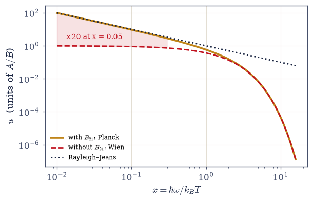
Fig. 686 The counterfactual with teeth. The equilibrium spectrum enforced by two-level atoms (in units of \(A/B\), against \(x = \hbar\omega/k_BT\)): with stimulated emission (amber) the steady state is exactly Planck; with \(B_{21} = 0\) (red dashed) it is Wien’s exponential. At large \(x\) the two agree — comparing there proves nothing (the stated trap). The classical Rayleigh–Jeans limit \(u \to 1/x\) (dark dotted) is where they part company: at \(x = 0.05\) the counterfactual sits a factor 20 below the classical demand (shaded gap). Equilibrium light without stimulated emission fails classical physics — which is how Einstein predicted a quantum process in 1917 without a quantum mechanics to derive it from (Eq. 772).

Validation 2

✓  without B21, equilibrium light fails the classical limit by a factor 20   [max|Δ| = 0.000438529 (rtol=0.02, atol=1e-09)]

True

Exercise 3 — The landscape: where light glows and where it amplifies

Stimulated/spontaneous \(= \bar n\), mapped. Cite Eq. 773.

1. Derive stimulated/spontaneous \(= B u/A = \bar n\) and the total-emission \((\bar n + 1)\) (the family reunion stated: the variance of §7.7, the ladder \(\sqrt{n+1}\), QED’s vacuum \(+1\)).

2. Write crossover_frequency(T) for the boundary this exercise is named after: setting \(\bar n = 1\) in \(1/(e^{h\nu/k_BT} - 1)\) gives \(\nu = (k_BT/h)\ln 2\), with glowing above it and amplifying below.

3. Evaluate it at 300 K, and compute \(\bar n\) for Na D (the float-ceiling guard stated), CO₂, and 21 cm with the Setup nbar — all via numpy.expm1.

4. Plot the \((\nu, T)\) plane with the \(\bar n = 1\) line and the three systems placed on it.

5. Read the map (prose): the optical world at everyday temperatures is spontaneous (hot things glow, never lase unaided) while the radio sky amplifies; masers before lasers, and astrophysical masers (OH, H₂O, SiO) glowing unpumped in stellar envelopes, named.

n̄ = 1 crossover at 300 K: ν = k_BT ln2/h = 4.33 THz
  Na D (589 nm)   x =      81.4   n̄ = 4.34e-36
  CO2 (10.6 um)   x =      4.52   n̄ = 0.011
  H I (21 cm)     x =  0.000227   n̄ = 4.4e+03

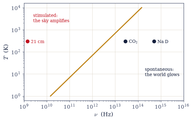
Fig. 687 Where light glows and where it amplifies. The \((\nu, T)\) plane divided by the line \(\bar n = 1\), i.e. \(h\nu = k_BT\ln 2\) (amber): above it spontaneous emission rules (\(\bar n \ll 1\) — hot matter glows; the optical world), below it stimulated emission rules (\(\bar n \gg 1\) — the radio universe amplifies). The three landmarks at 300 K: sodium D at \(\bar n \sim 4\times10^{-36}\), the CO₂ laser line at 0.011, and the 21-cm hyperfine line at 4400 (Eq. 773). The map explains the history: masers (1954) preceded lasers (1960) because the radio sky is already half-way to amplification, and astrophysical OH/H₂O/SiO masers glow unpumped in stellar envelopes while nature builds no optical laser at all.

Validation 3

✓  the n̄ landscape: glow above the ln2 line, amplify below it   [max|Δ| = 0.344381 (rtol=0.02, atol=1e-09)]
✓  and the optical world is spontaneous to one part in 10^36   [max|Δ| = 4.05786e-05 (rtol=0.08, atol=1e-09)]

True

Exercise 4 — The two-level no-go

Drive a two-level atom as hard as physics allows: it equalizes and stops. Cite Eq. 774.

1. Solve the driven steady state from flow balance, \(N_2/N_1 = Bu/(A + Bu)\), and show it is \(< 1\) for every finite drive.

2. Write steady_two_level(drive) returning that ratio as a function of the dimensionless drive \(s = Bu/A\) — the no-go this exercise is named for, made callable.

3. Verify the saturation numerically across \(Bu/A = 0.1 \to 10^4\) and plot the approach.

4. Attribute the verdict (prose): absorption and stimulated emission are one matrix element read both ways (the forced \(g_1B_{12} = g_2B_{21}\)); the same symmetry that made Planck work forbids two-level gain; saturation named as the two-level system’s universal response (the Rabi physics of §6.24, one breath).

5. Pose the engineering question the next exercise answers: if not two levels, how many?

  Bu/A =      0.1:  N2/N1 = 0.0909
  Bu/A =      1.0:  N2/N1 = 0.5000
  Bu/A =     10.0:  N2/N1 = 0.9091
  Bu/A =    100.0:  N2/N1 = 0.9901
  Bu/A =  10000.0:  N2/N1 = 0.9999

ceiling verified: N2/N1 < 1 for all drives (max 0.9999 at Bu/A = 1e4)

Validation 4

✓  the two-level no-go: monotone saturation strictly below equalization, under any drive   [N2/N1 = 0.9999 at Bu/A = 1e4]
✓  the saturation curve's two ends, on their stated values   [max|Δ| = 9.09091e-06 (rtol=0.01, atol=1e-09)]

True

Exercise 5 — Three levels, four levels: the pumping economics

Ruby’s brutal cost and Nd:YAG’s easy terms — by flow balance. The three-level (ruby) scheme pumps \(1\to3\), decays fast (\(S\)) \(3\to2\), and lases (\(A\)) \(2\to1\) into the ground state; the four-level scheme pumps \(0\to3\), decays fast \(3\to2\), lases \(2\to1\), and drains fast \(1\to0\). Throughout \(A = 1\) and \(S = 1000\), the fast-band hierarchy \(S \gg A\). Each steady state closes on the conservation row \(\sum_i N_i = 1\) — dropping the pump band from the normalization because “\(S\) is fast, so \(N_3 \approx 0\)” is the stated trap, silently inflating the inversion near onset. Cite Eq. 775.

1. Write steady_three_level(P, A=1.0, S=1000.0) returning \((N_1, N_2, N_3)\): solve the balances \(PN_1 = SN_3\) and \(SN_3 = AN_2\) together with \(\sum N = 1\) in closed form. Write this one yourself — the implementation is the lesson.

2. Write rate_matrix_steady(rates, n_levels), the general route: assemble \(\dot N = M\,N\) from a list of \((i, j, \text{rate})\) transitions (population flows \(i \to j\) at \(\text{rate}\cdot N_i\)), replace the last, redundant balance row of \(M\) with the conservation row, and solve with numpy.linalg.solve. Write this one yourself — the implementation is the lesson.

3. Solve the three-level steady state by both routes, verifying \(\sum N = 1\) explicitly and the two routes against each other at \(10^{-10}\).

4. Verify: inversion \(N_2 > N_1\) exactly when \(P > A\), with onset at \(N_2 = 1/2\): more than half of all atoms held aloft (Maiman’s flashlamp, one sentence).

5. Write steady_four_level(P, A=1.0, S=1000.0) returning \((N_0, N_1, N_2, N_3)\) for the four-level chain, again in closed form with \(\sum N = 1\). Write this one yourself — the implementation is the lesson.

6. Verify inversion at any pump (\(P/A = 0.01\); Nd:YAG named), cross-check it against your Part 2 rate_matrix_steady, and plot inversion vs pump for two-, three-, and four-level schemes on one axes.

7. Read the economics (prose): the lower laser level is the whole game. Ruby lases into its ground state and pays a heavy price for it; four-level designs lase into a level that empties itself; why nearly every practical laser is four-level.

three-level at P = 1.7: N = (0.3701, 0.6292, 0.0006),  ΣN = 1.000000000000
closed form vs numpy.linalg.solve: max gap = 1.1e-16

three-level onset (P = A): N2 = 0.4998 (the half-population price), ΣN = 1.000000000000

four-level at P/A = 0.01: N2 − N1 = 0.00989 > 0,  ΣN = 1.000000000000
closed form vs linalg route: max gap = 1.1e-16

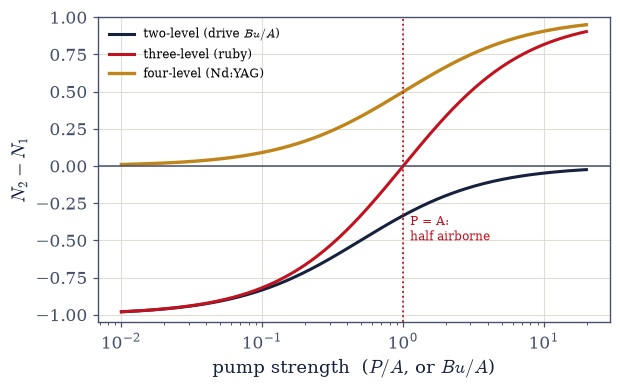
Fig. 688 The pumping economics of inversion. Population difference \(N_2 - N_1\) of the lasing pair against pump strength for the three classic schemes, by steady-state flow balance (closed forms cross-checked against numpy.linalg.solve at \(10^{-12}\)). Two levels (dark): the difference saturates at zero from below — equalization is the ceiling, the no-go of Exercise 4. Three levels (red, ruby): inversion begins only at \(P = A\), where half of all atoms are already airborne — the flashlamp price Maiman paid in 1960. Four levels (amber, Nd:YAG): the lower laser level drains itself, so any pump inverts — the design choice behind nearly every practical laser (Eq. 775). The lower laser level is the whole game.

Validation 5

✓  the pumping economics: ruby's half-population onset; four levels invert for pocket change   [max|Δ| = 0.000249875 (rtol=0.02, atol=1e-09)]
✓  conservation held explicitly in both schemes: no population lost to the dropped-band trap   [|ΣN − 1| = 2.2e-16]
✓  closed-form flow balance and the general linalg solve agree   [max gaps 1.1e-16, 1.1e-16]

True

Exercise 6 — Negative temperature, the promise kept

The inverted medium given the temperature §7.4 promised it. Cite Eq. 776.

1. Derive \(T = -\hbar\omega/[k_B\ln(g_1N_2/g_2N_1)]\) from the Boltzmann ratio read backwards.

2. Write negative_T(ratio, nu_Hz) for that assignment at \(g_1 = g_2\) — the temperature this exercise is named for, made callable.

3. Verify the ladder (ratios 0.5, 0.9, 1.5, 3.0 at the ruby line) and plot \(T(N_2/N_1)\) with the \(\beta\)-axis inset.

4. Teach the ordering via the \(\beta\)-picture of §7.4 (prose + the inset): \(\beta\) falls smoothly through zero; deeper inversion brings \(T\) toward \(0^-\), a scale that is upside down on purpose.

5. State the payoff (prose): hotter than every positive temperature means net energy flows from the medium to any beam; gain is a thermodynamic status, not just a rate inequality; the bounded-spectrum requirement of §7.4 re-invoked.

  N2/N1 = 0.5:  T =    +29897 K
  N2/N1 = 0.9:  T =   +196684 K
  N2/N1 = 1.5:  T =    -51108 K
  N2/N1 = 3.0:  T =    -18863 K

the same ladder in β (1/K): [ 3.34e-05  5.08e-06 -1.96e-05 -5.30e-05]
monotone through zero — the β-axis tells the story straight

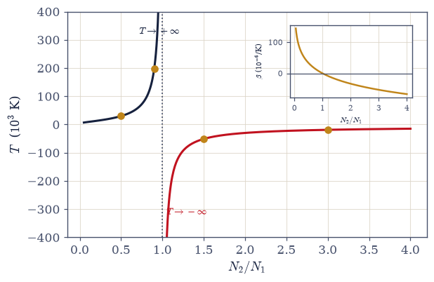
Fig. 689 The temperature of a gain medium. Boltzmann temperature of a two-level population pair against its ratio \(N_2/N_1\) at the ruby line (Eq. 776): ordinary positive temperatures below equalization, a divergence to \(\pm\infty\) at it, and negative temperatures beyond — with deeper inversion bringing \(T\) toward \(0^-\) (\(N_2/N_1 = 1.5\) reads \(-51\,000\) K). Inset: the same ladder on the \(\beta\)-axis of §7.4, where the story is smooth and monotone: \(\beta\) falls through zero and keeps going; the temperature scale is upside down on purpose, an artifact of the \(1/\beta\) lens. A medium at negative temperature is hotter than every positive-temperature system, which is why it gives net energy to any beam it meets — gain as a thermodynamic status.

Validation 6

✓  the gain medium's negative temperature: N2/N1 = 1.5 at the ruby line   [got -51108.5 vs expected -51131 (rtol=0.01, atol=1e-09)]
✓  and the β-axis tells it straight: monotone through zero as inversion deepens

True

Exercise 7 — The ω³ tyranny

Sixteen nanoseconds versus eleven million years, decomposed honestly. Cite Eq. 777.

1. State \(A = (\hbar\omega^3/\pi^2c^3)B\) and its consequence: lifetimes plummet as the cube of frequency.

2. Compute the ratio \(A(\text{Na D})/A(\text{21 cm})\) from the cited values, and \(\tau(21\text{ cm})\) in years.

3. Decompose: \((\nu_{\text{Na}}/\nu_{21})^3\) against the residual (the forced law’s 16.7 orders versus the hyperfine flip’s magnetic-dipole forbiddenness); attribute each honestly.

4. Spend the result (prose, outward): the 21-cm line survives 11 Myr and therefore maps the galaxy; X-ray lasing fights an \(\omega^3\) headwind. One sentence each.

A(Na D)/A(21 cm) = 2.16e+22   (log10 = 22.3)
τ(Na D) = 16.2 ns;   τ(21 cm) = 11.1 Myr

ω³ law:          16.7 orders   (the forced A/B ∝ ω³)
matrix element:  5.7 orders   (magnetic-dipole forbiddenness)

Validation 7

✓  the ω³ tyranny, decomposed: the forced law's 16.7 orders, the matrix element's 5.7   [max|Δ| = 0.0371213 (rtol=0.02, atol=1e-09)]
✓  eleven million years: the lifetime that lets 21-cm light map the galaxy   [got 1.11178e+07 vs expected 1.11e+07 (rtol=0.05, atol=1e-09)]

True

Exercise 8 — The minimal laser

One mode, one reservoir, one kink. Cite Eq. 778.

1. Assemble \(dn/dt = GN_2(n + 1) - n/\tau_c\) and \(dN_2/dt = P - AN_2 - GnN_2\); identify the \(+1\) as the spontaneous seed (Exercise 3’s family, at work).

2. Write laser_steady_state(P, G=0.01, A=1.0, tau_c=10.0) returning \((n, N_2)\): eliminate \(N_2 = P/(A + Gn)\) from the photon equation, then root-find the remaining residual in \(n\) with scipy.optimize.brentq on the deliberately asymmetric bracket \([10^{-12}, 10^9]\) (below threshold the root is a spontaneous-seeded sliver, above it macroscopic, so a symmetric bracket around \(n \sim 1\) misses one regime). Write this one yourself — the implementation is the lesson.

3. Scan it across \(P\) and locate the threshold \(P_{\text{th}} = A/G\tau_c = 10\).

4. Verify the two signatures: \(N_2\) clamps at \(1/G\tau_c = 10\) above threshold while \(n\) rises linearly as \((P - P_{\text{th}})\tau_c\); plot both with the kink.

5. Name the physics (prose): gain clamping as the laser’s defining feedback (the medium refuses to hold more inversion than the cavity spends), and the threshold as a nonequilibrium phase transition, one breath toward the volume’s closing questions.

P_th = A/(Gτ_c) = 10
below (P = 5):  n = 0.98   (spontaneous-seeded glow)
above (P = 30): n = 201.5,  N2 = 9.95  (clamp at 1/Gτ_c = 10)
linear law at P = 30: (P − P_th)τ_c = 200 vs solved 201.5

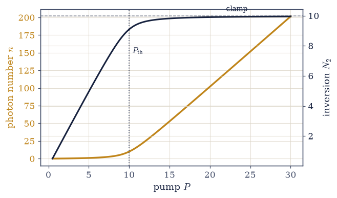
Fig. 690 The kink and the clamp. Steady state of the minimal single-mode laser (Eq. 778; \(G = 0.01\), \(A = 1\), \(\tau_c = 10\), so \(P_{\text{th}} = 10\)), solved by brentq on the asymmetric bracket \([10^{-12}, 10^9]\). Left axis (amber): photon number — a spontaneous-seeded floor below threshold (the \(+1\)’s quiet work), then a linear rise \(n = (P - P_{\text{th}})\tau_c\) above it (201 at \(P = 30\)). Right axis (dark): the inversion \(N_2\) grows linearly below threshold, then clamps at \(1/G\tau_c = 10\) — the medium refuses to hold more gain than the cavity spends, and every additional pump quantum becomes light. The kink is a nonequilibrium phase transition: an order parameter rising from a fluctuation floor at a sharp pump value.

Validation 8

✓  threshold: the kink and the clamp   [max|Δ| = 0.488916 (rtol=0.03, atol=1e-09)]
✓  gain clamping: the inversion pins at 1/Gτ_c above threshold   [got 9.95061 vs expected 9.95 (rtol=0.01, atol=1e-09)]
✓  and below threshold only the spontaneous seed glows   [n(P = 5) = 0.98]

True

Exercise 9 — The argument that outran its mechanics

Everything in this notebook flowed from refusing to let atoms disagree with light. Einstein wrote three rates he could not derive, demanded they reproduce a law he could not doubt, and the demand did the deriving: absorption and stimulated emission locked to one matrix element, spontaneous emission priced at \(\hbar\omega^3/\pi^2c^3\), and a new process conjured into existence because the classical limit would fail without it. A century of consequences followed on schedule: the maser where \(\bar n\) is large, the laser where engineering supplies what temperature will not, ruby paying its half-population price while four-level designs invert for pocket change, and a rod of chromium ions sitting, briefly, at fifty thousand kelvin below zero.

It is worth noticing what kind of argument this was. No Hamiltonian, no wavefunction, no matrix element: just equilibrium, held to strictly. Thermodynamics cannot tell you what the rates are; it can tell you what they must be consistent with, and sometimes, as here, consistency has exactly one solution. Einstein trusted that, and predicted a machine his century could not yet build.

The movement’s gas now has its conversation with matter. Next, the same statistics moves into a solid: the crystal as a box of phonon modes, Debye’s \(T^3\), and the low-temperature law that §7.10 invoked on trust, derived at last (§7.16).

Notebook summary

Matter in equilibrium with the gas of §7.14, and thermodynamics run in reverse.

• The forced relations Eq. 771, Eq. 772: three 1917 postulates, one steady state, and Planck’s law leaving no freedom: \(g_1B_{12} = g_2B_{21}\) and \(A/B_{21} = \hbar\omega^3/\pi^2c^3\); the balance solved numerically by brentq lands on the analytic Planck form at \(10^{-10}\) (gated).

• The counterfactual — without \(B_{21}\) the steady state is Wien, failing the classical limit by 20× at \(x = 0.05\) (\(u\cdot x = 0.048\) vs 0.975, gated; the small-\(x\)-only comparison explained): stimulated emission predicted from consistency, 43 years before Maiman.

• The landscape Eq. 773: stimulated/spontaneous \(= \bar n\) exactly (one family with the bunching of §7.7 and the ladder \(\sqrt{n+1}\)); crossover at \(k_BT\ln2/h = 4.33\) THz (gated); Na D at \(4\times10^{-36}\), CO₂ at 0.011, 21 cm at 4400 (gated): the optical world glows, the radio sky amplifies, masers before lasers.

• The no-go Eq. 774: \(N_2/N_1 = s/(1+s) < 1\) always (monotone saturation gated to 0.9999 at \(s = 10^4\)): one matrix element, two directions.

• The economics Eq. 775: ruby inverts only past \(P = A\) with half the medium airborne; four levels invert at \(P/A = 0.01\) (both gated); conservation and the closed-form-vs-linalg.solve cross-check gated at \(10^{-10}\).

• Negative temperature Eq. 776: the promise §7.4 planted, kept: \(N_2/N_1 = 1.5\) reads \(-51\,000\) K at the ruby line (gated), with the \(\beta\)-axis monotone through zero (gated): gain as a thermodynamic status.

• The ω³ tyranny Eq. 777: 22.3 orders between Na D and 21 cm, decomposed: 16.7 forced by \(\omega^3\), 5.7 from magnetic-dipole forbiddenness (gated); eleven million years is why the galaxy can be mapped in hydrogen light.

• The minimal laser Eq. 778: threshold at \(P_{\text{th}} = A/G\tau_c\), the inversion clamping at \(1/G\tau_c\) while \(n\) rises linearly (kink, clamp, and seed all gated): a nonequilibrium phase transition, named.

Next door the same statistics moves into a crystal: phonons and Debye’s \(T^3\).

Outlook

• Phonons and Debye (§7.16). The same mode-counting in a crystal; the \(T^3\) law that §7.10 invoked on trust, derived where it belongs.

• BEC (§7.17). Bosonic amplification of matter waves: the atom laser, named.

• Outward horizons, named. QED’s derivation of \(A\) (vacuum fluctuations; the \(+1\) at \(n = 0\)); Rabi oscillations and saturation spectroscopy; astrophysical masers and the 21-cm sky.

• Cross-reference §7.14 (the gas; Planck non-negotiable), §7.4 (the Boltzmann ratio; the negative-temperature seed, grown here), §7.7 (the \((n+1)\) family), §6.24 (the golden rule for \(B\)), §7.5 (the oscillator per mode).

Take this notebook with you

Use the download button (↓) in the toolbar above to save this notebook and run it yourself. The published notebooks ship without worked solutions; if you would like the reference solutions — to teach from or to check your own work — get in touch: hello@ramador.me.