6.2 Linear Operators, Hermitian and Unitary Operators, and the Spectral Theorem

Elementary Computational Physics

Volume VI — Quantum Mechanics Notebook 6.2

The actors. With the stage built, we introduce what acts on it: linear operators. Two kinds run all of quantum mechanics — Hermitian operators, whose real eigenvalues are the things we can measure, and unitary operators, which move states around without disturbing probabilities. The spectral theorem ties them together and hands us the one computation we will run all volume: diagonalization.

Level · advanced   •   Est. · 160–200 min

Raymond Amador v1.4.0  ·  2026-07-31  ·  CC BY 4.0 (text) / MIT (code)

Notebook overview

In §6.1 we built the stage — the complex Hilbert space, where a quantum state is a unit vector. This notebook brings on the actors: the linear operators that act on those states. It is the heaviest notebook of Movement 0 and the most important, because it contains the single sentence that the rest of the volume is a commentary on — quantum mechanics is linear algebra on a complex Hilbert space. Once that is computational, so is everything built from it.

Two classes of operator carry the entire theory, and the notebook is organized around them. The first is the Hermitian operators, those equal to their own adjoint, \(A=A^{\dagger}\). We will prove — gently, but actually prove — that a Hermitian operator has real eigenvalues and an orthonormal eigenbasis. These two facts are exactly what an observable needs: real eigenvalues are the possible results of a measurement, and the orthonormal eigenvectors are the states with a definite value. The second class is the unitary operators, those satisfying \(U^{\dagger}U=I\). They preserve the inner product, hence norms, hence probabilities — which is precisely what a symmetry or a time evolution must do, since a state has to stay normalized. Their eigenvalues lie on the unit circle.

Binding the two classes is the spectral theorem: every Hermitian operator can be written \(A=V\Lambda V^{\dagger}\), a diagonal matrix \(\Lambda\) of real eigenvalues conjugated by a unitary \(V\) of orthonormal eigenvectors. This is the master computation of the volume — to understand a Hermitian operator, diagonalize it — and numpy.linalg.eigh is its engine. A short bridge, the exponential map \(U=e^{-iH}\), turns a Hermitian operator into a unitary one and previews the deepest structural fact of dynamics: the Hamiltonian (a Hermitian observable) generates time evolution (a unitary). We close with commuting operators, which share an eigenbasis and so are the compatible observables, the ones that can be sharp at once.

As in every Volume VI notebook, each exercise opens with a crystal-clear statement and explicit enumerated parts that name the exact operation to run — numpy.linalg.eigh versus numpy.linalg.eig, A.conj().T for the adjoint, scipy.linalg.expm for the matrix exponential, the @ operator for composition — so the method is never something to reverse-engineer. The difficulty lives in the mathematics, never in deciphering the question.

A word on notation (and its boundary). We write the spectral theorem here as a matrix factorization, \(A=V\Lambda V^{\dagger}\), obtained by diagonalization. Its equivalent and more eloquent form as a sum of projectors, \(A=\sum_\lambda \lambda\,|\lambda\rangle\langle\lambda|\), together with the general machinery of functions of operators \(f(A)=\sum_\lambda f(\lambda)\,|\lambda\rangle\langle\lambda|\), is the work of §6.3, once Dirac notation gives us the outer product \(|\lambda\rangle\langle\lambda|\) as an object. We use the exponential map \(U=e^{-iH}\) concretely here, via scipy.linalg.expm; its place in the general theory is §6.3, and time evolution proper is §6.7.

How to read the checks. Each exercise closes with a validate call against an independent fact: that operators compose by matrix multiplication and generally fail to commute; the adjoint identity \(\langle u|A^{\dagger}v\rangle=\langle Au|v\rangle\); a Hermitian operator’s real spectrum and orthonormal eigenbasis; the factorization \(A=V\Lambda V^{\dagger}\) to machine precision; a unitary’s inner-product preservation and unit-circle spectrum; that \(e^{-iH}\) is unitary with eigenvalues \(e^{-i\lambda}\); that commuting operators share an eigenbasis; and the Pauli algebra. A ✓ is strong evidence; a ✗ is a prompt to locate the discrepancy.

Scope. Operators on a finite-dimensional complex space, and the spectral theorem in matrix form. Dirac notation and the projector form are §6.3; the measurement postulate (eigenvalues as outcomes, \(|\langle\lambda|\psi\rangle|^2\) as probabilities) is §6.5; commutators and uncertainty are §6.6; time evolution is §6.7. See Sakurai & Napolitano (Ch. 1); Nielsen & Chuang; Axler; and Notebooks §6.1 (the inner-product space), §0.4–§0.5 (eigenvalue problems).

Theory in brief

Linear operators as matrices

A linear operator \(A\) sends states to states linearly, \(A(a|u\rangle+b|v\rangle)=aA|u\rangle+ bA|v\rangle\). In an orthonormal basis it is a matrix, with entries the inner products

(494)\[A_{ij}=\langle e_i|A|e_j\rangle,\qquad (A|\psi\rangle)_i=\sum_j A_{ij}\psi_j ,\]

so acting on a state is matrix–vector multiplication and composing operators is matrix multiplication (@). Unlike numbers, operators generally do not commute, \(AB\ne BA\) — a fact we flag now and build the whole theory of measurement on later.

The adjoint

The adjoint \(A^{\dagger}\) is defined by \(\langle u|A^{\dagger}v\rangle=\langle Au|v\rangle\) for all \(u,v\). In an orthonormal basis it is the conjugate transpose,

(495)\[A^{\dagger}=(A^{*})^{\mathsf T}\quad(\texttt{A.conj().T}),\qquad (A^{\dagger})^{\dagger}=A,\quad (AB)^{\dagger}=B^{\dagger}A^{\dagger} .\]

It is the operator analogue of complex conjugation, and the order reverses under a product.

Hermitian operators — the observables

An operator is Hermitian (self-adjoint) if \(A=A^{\dagger}\). Two theorems follow, and both are proved gently in the exercises:

(496)\[A=A^{\dagger}\ \Longrightarrow\ \text{eigenvalues real},\quad \text{eigenvectors of distinct eigenvalues orthogonal} .\]

Real eigenvalues: if \(A|\lambda\rangle=\lambda|\lambda\rangle\) then \(\langle\lambda|A|\lambda\rangle =\lambda\langle\lambda|\lambda\rangle\); but \(\langle\lambda|A|\lambda\rangle\) equals its own conjugate (because \(A=A^{\dagger}\)), so it is real, and \(\langle\lambda|\lambda\rangle>0\) is real — hence \(\lambda\) is real. Orthogonal eigenvectors: for \(A|a\rangle=a|a\rangle\), \(A|b\rangle=b|b\rangle\) with \(a\ne b\), computing \(\langle b|A|a\rangle\) two ways gives \((a-b)\langle b|a\rangle=0\), so \(\langle b|a\rangle=0\). A Hermitian operator therefore has an orthonormal eigenbasis. Physically, Hermitian operators are the observables: real eigenvalues are the possible measurement results, orthonormal eigenvectors the definite-value states (the measurement postulate is §6.5). numpy.linalg.eigh is the tool — it exploits \(A=A^{\dagger}\) to return real eigenvalues and orthonormal eigenvectors, where the general numpy.linalg.eig would not.

The spectral theorem

Collecting the orthonormal eigenvectors as the columns of a matrix \(V\) and the real eigenvalues on the diagonal of \(\Lambda\), the eigenvalue equation \(AV=V\Lambda\) rearranges into the spectral theorem,

(497)\[A=V\Lambda V^{\dagger},\qquad V\ \text{unitary},\quad \Lambda=\operatorname{diag}(\lambda_1,\dots,\lambda_n)\ \text{real} .\]

To understand a Hermitian operator, diagonalize it. (The projector form \(A=\sum_\lambda\lambda\, |\lambda\rangle\langle\lambda|\) is §6.3.)

Unitary operators — the symmetries and dynamics

An operator is unitary if \(U^{\dagger}U=I\) (so \(U^{\dagger}=U^{-1}\)). Unitary operators preserve the inner product, and therefore probabilities,

(498)\[U^{\dagger}U=I\ \Longrightarrow\ \langle Uu|Uv\rangle=\langle u|v\rangle,\quad \|U\psi\|=\|\psi\|,\quad |\lambda_j(U)|=1 .\]

Their eigenvalues lie on the unit circle. Physically, unitary operators are the symmetries (rotations, reflections, basis changes) and the dynamics (time evolution is unitary, §6.7).

The exponential map: from Hermitian to unitary

The two classes are linked by the exponential. For Hermitian \(H\),

(499)\[U=e^{-iH}\ \text{is unitary},\qquad \text{eigenvalues } e^{-i\lambda_j}\ \text{on the unit circle} ,\]

which we compute with scipy.linalg.expm. This is the seed of dynamics: a Hermitian observable — the Hamiltonian, energy — generates a unitary, \(U(t)=e^{-iHt/\hbar}\) (§6.7).

Commuting operators share an eigenbasis

The commutator is \([A,B]=AB-BA\). If two Hermitian operators commute, they are simultaneously diagonalizable (Sakurai & Napolitano, §1.4, supply the proof; Exercise 7 verifies it numerically),

(500)\[[A,B]=0\ \Longleftrightarrow\ A,B\ \text{share a common orthonormal eigenbasis} ,\]

the statement that commuting observables are compatible — they can have simultaneously definite values. Non-commuting observables, by contrast, obey an uncertainty relation (§6.6).

Setup

Data and instruments only: the series palette, the three Pauli matrices, and the small certification predicates and library wrappers the exercises grade their results against — is_hermitian, is_unitary, the numpy.linalg.eigh wrapper spectral_decomposition, and commutator. The one operation the whole notebook is written in terms of, the adjoint \(A^{\dagger}=\)A.conj().T, is deliberately not here: you write it in Exercise 2, which is named for it, and the predicates below call it from there.

The Setup below holds this notebook’s data and instruments — nothing you are asked to build. It is collapsed so the building stays yours; expand it whenever you want the details.

Show code cell source

Hide code cell source

import matplotlib.pyplot as plt
import numpy as np
from scipy.linalg import expm

from ecp import draw, validate

ACCENT, INK, SOFT = draw.ACCENT, draw.INK, draw.SOFT  # data: the series palette

# Conventions: operators are matrices in a fixed orthonormal basis of finite-dimensional
# ℂⁿ; the adjoint A† is the conjugate transpose A.conj().T; the inner product ⟨u|v⟩ = numpy.vdot(u, v)
# (conjugate-first, from §6.1). We diagonalize Hermitian operators with numpy.linalg.eigh (real spectra,
# orthonormal eigenvectors) — NOT numpy.linalg.eig, which is for general matrices and returns neither.

# data: the Pauli matrices — the canonical Hermitian operators, used throughout (and the spin
# observables of Movement I)
SX = np.array([[0, 1], [1, 0]], dtype=complex)
SY = np.array([[0, -1j], [1j, 0]], dtype=complex)
SZ = np.array([[1, 0], [0, -1]], dtype=complex)


# instrument: a certification predicate, not the lesson — the lesson is what Hermiticity
# implies, not how to test for it. It calls the `adjoint` you write in Exercise 2, which
# Python resolves at call time.
def is_hermitian(A, tol=1e-12):
    """Test whether ``A`` is Hermitian, $A=A^{\\dagger}$ {eq}`eq-hermitian`.

    Compares ``A`` with its conjugate transpose (``A.conj().T``) using ``numpy.allclose``. A Hermitian
    operator is an observable: its eigenvalues (real) are the possible measurement outcomes.

    Parameters
    ----------
    A : numpy.ndarray
        A square complex matrix.
    tol : float, optional
        Absolute tolerance passed to ``numpy.allclose``.

    Returns
    -------
    bool
        ``True`` if ``A`` equals its adjoint to within ``tol``.
    """
    return np.allclose(A, adjoint(A), atol=tol)


# instrument: the companion certification predicate for unitarity; like `is_hermitian` it
# calls the Exercise 2 `adjoint`, resolved at call time.
def is_unitary(U, tol=1e-12):
    """Test whether ``U`` is unitary, $U^{\\dagger}U=I$ {eq}`eq-unitary`.

    Checks that the adjoint times the operator is the identity, via ``numpy.allclose(U.conj().T @ U,
    numpy.eye(n))``. A unitary operator preserves inner products and hence probabilities — the
    symmetries and the dynamics.

    Parameters
    ----------
    U : numpy.ndarray
        A square complex matrix.
    tol : float, optional
        Absolute tolerance passed to ``numpy.allclose``.

    Returns
    -------
    bool
        ``True`` if $U^{\\dagger}U=I$ to within ``tol``.
    """
    n = U.shape[0]
    return np.allclose(adjoint(U) @ U, np.eye(n), atol=tol)


# instrument: a naming wrapper over the `numpy.linalg.eigh` dispatch — the LAPACK engine is a
# given tool (§0.5), and the spectral factorization H = VΛV† it feeds is assembled in Exercise 4.
def spectral_decomposition(H):
    """Diagonalize a Hermitian operator, $H=V\\Lambda V^{\\dagger}$ {eq}`eq-ops-spectral`.

    Wraps ``numpy.linalg.eigh``, which exploits Hermiticity to return **real** eigenvalues (ascending)
    and an **orthonormal** matrix of eigenvectors ``V`` (the eigenvectors are its columns). The matrix
    form $H=V\\Lambda V^{\\dagger}$ returned here is recast as a sum of projectors $H=\\sum_\\lambda
    \\lambda|\\lambda\\rangle\\langle\\lambda|$ in §6.3.

    Parameters
    ----------
    H : numpy.ndarray
        A Hermitian matrix.

    Returns
    -------
    eigenvalues : numpy.ndarray
        The real eigenvalues, ascending.
    V : numpy.ndarray
        The unitary matrix whose columns are the orthonormal eigenvectors.
    """
    eigenvalues, V = np.linalg.eigh(H)
    return eigenvalues, V


# data: the definition [A,B] = AB − BA transcribed — a given expression, not machinery; the
# lesson of Exercises 7 and 8 is what its vanishing (and non-vanishing) means.
def commutator(A, B):
    """The commutator $[A,B]=AB-BA$ {eq}`eq-commute`.

    Computed with the matrix-multiply operator ``@``. It vanishes exactly when $A$ and $B$ share a
    common eigenbasis — the algebraic signature of *compatible* observables.

    Parameters
    ----------
    A, B : numpy.ndarray
        Square matrices of equal shape.

    Returns
    -------
    numpy.ndarray
        The commutator ``A @ B - B @ A``.
    """
    return A @ B - B @ A

Exercise 1 — Operators as matrices

In an orthonormal basis a linear operator is a matrix: acting on a state is the matrix–vector product, and composing two operators is matrix multiplication Eq. 494. Let \(A\) and \(B\) be the two operators on \(\mathbb{C}^4\) given below, and let \(|\psi\rangle=(1,\ i,\ 0,\ 2)^{\mathsf T}\). Unlike numbers, matrices need not commute, and this pair is generic in that respect — the failure of \(AB=BA\) is not an accident of these entries but the algebraic fact the whole theory of measurement is later built on.

1. Build the matrices \(A\) and \(B\) as complex numpy.ndarrays and the state \(|\psi \rangle\).

2. Act on the state with the matrix–vector product A @ psi.

3. Verify linearity by checking A @ (a*u + b*v) equals a*(A @ u) + b*(A @ v) with numpy.allclose.

4. Compose the operators both ways with A @ B and B @ A and confirm they differ (numpy.allclose(A @ B, B @ A) is False) — operators are matrices, and matrices need not commute.

A|ψ⟩ = [1.+0.j 2.+0.j 0.+2.j 0.+1.j]
linear: A(a|u⟩+b|v⟩) = a A|u⟩ + b A|v⟩ ?  True
AB = BA ?  False   (so AB ≠ BA: True)
  ‖AB − BA‖ = 5.657

Validation 1

✓  operators are matrices acting on states by matrix multiplication, and they need not commute (AB ≠ BA)

True

Exercise 2 — The adjoint and its algebra

The adjoint \(A^{\dagger}\) is defined abstractly by \(\langle u|A^{\dagger}v\rangle=\langle Au|v\rangle\) for all \(u,v\); in an orthonormal basis it is the conjugate transpose \((A^{*})^{\mathsf T}\) Eq. 495. It is the operator analogue of complex conjugation, and it carries an algebra of its own: applying it twice returns the original operator, and it reverses the order of a product, \((AB)^{\dagger}=B^{\dagger}A^{\dagger}\). Everything the rest of this notebook says about Hermitian and unitary operators is written in terms of this one operation, so it is the piece you build. The operators \(A,B\) and the vectors \(u,v\) are those of Exercise 1.

1. Write adjoint(A), returning the conjugate transpose A.conj().T.

2. Apply it to the operator \(A\) of Exercise 1 to form \(A^{\dagger}\).

3. Verify the defining property: compute \(\langle u|A^{\dagger}v\rangle\) as numpy.vdot(u, adjoint(A) @ v) and \(\langle Au|v\rangle\) as numpy.vdot(A @ u, v), and compare them.

4. Verify the algebra with numpy.allclose: that adjoint(adjoint(A)) equals A, and that adjoint(A @ B) equals adjoint(B) @ adjoint(A) (note the order reverses).

⟨u|A†v⟩ = 0.0000+2.0000j
⟨Au|v⟩  = 0.0000+2.0000j   (equal: True)
(A†)† = A ?  True
(AB)† = B†A† ?  True   (and (AB)† = A†B† ?  False — the order matters)

Validation 2

✓  the adjoint satisfies its defining property ⟨u|A†v⟩ = ⟨Au|v⟩   [got 2j vs expected 2j (rtol=1e-12, atol=1e-09)]
✓  the adjoint algebra holds: (A†)† = A and (AB)† = B†A† (the order reverses)

True

Exercise 3 — Hermitian operators: real eigenvalues and an orthonormal eigenbasis

Two theorems make Hermitian operators, \(H=H^{\dagger}\), the observables of the theory Eq. 496, and both have short proofs. The eigenvalues are real because \(\langle\lambda|H|\lambda\rangle\) is at once \(\lambda\langle\lambda|\lambda\rangle\) and its own complex conjugate, while \(\langle\lambda|\lambda\rangle>0\) is real. Eigenvectors belonging to distinct eigenvalues are orthogonal because computing \(\langle b|H|a\rangle\) two ways gives \((a-b)\langle b|a\rangle=0\). Together they say a Hermitian operator has an orthonormal eigenbasis — real possible outcomes, and a definite-value state for each of them.

1. Build a Hermitian \(H\) by symmetrizing a random complex matrix, H = M + M.conj().T (this guarantees \(H=H^{\dagger}\); use the adjoint you wrote in Exercise 2, and confirm with the is_hermitian helper).

2. Diagonalize with numpy.linalg.eigh (the spectral_decomposition helper) — not numpy.linalg.eig, because eigh is built for Hermitian matrices and returns real eigenvalues and orthonormal eigenvectors.

3. Confirm the eigenvalues are real (eigh returns a real array) and the eigenvector matrix is orthonormal, \(V^{\dagger}V=I\) (numpy.allclose(adjoint(V) @ V, numpy.eye(4))).

is_hermitian(H) ?  True
eigenvalues (all real): [-3.4299 -1.4705  1.5777  3.7121]
eigenvectors orthonormal, V†V = I ?  True

Validation 3

✓  a Hermitian operator has real eigenvalues and an orthonormal eigenbasis — the mathematical signature of an observable

True

Exercise 4 — The spectral theorem: diagonalization

Collect a Hermitian operator’s orthonormal eigenvectors as the columns of a matrix \(V\) and its real eigenvalues on the diagonal of \(\Lambda\), and the eigenvalue equation \(HV=V\Lambda\) rearranges into the spectral theorem \(H=V\Lambda V^{\dagger}\), with \(V\) unitary Eq. 497. To understand a Hermitian operator, diagonalize it — this is the master computation of the volume, and the eigenvalues and eigenvector matrix it needs are already in hand from Exercise 3.

1. Take the eigenvalues and eigenvector matrix \(V\) from numpy.linalg.eigh (already computed in Exercise 3).

2. Form the diagonal matrix \(\Lambda\) with numpy.diag(eigenvalues).

3. Reconstruct \(V\Lambda V^{\dagger}\) with the matrix products V @ Lam @ adjoint(V) — the adjoint you wrote in Exercise 2 — and compare it to \(H\) via numpy.max(numpy.abs(H - V @ Lam @ adjoint(V))).

4. Separately confirm the eigenvalue equation H @ V equals V @ Lam with numpy.allclose, and that \(V\) is unitary (is_unitary(V)) — the change of basis that diagonalizes \(H\).

spectral theorem H = VΛV†:  max|H − VΛV†| = 2.4e-15
eigenvalue equation HV = VΛ ?  True
V unitary (the diagonalizing change of basis) ?  True

Validation 4

✓  the spectral theorem: every Hermitian operator factorizes as H = VΛV† with V unitary and Λ real diagonal   [got 2.44249e-15 vs expected 0 (rtol=1e-06, atol=1e-12)]

True

Exercise 5 — Unitary operators: the symmetries and dynamics

A unitary operator satisfies \(U^{\dagger}U=I\), so \(U^{\dagger}=U^{-1}\), and three consequences follow that together make unitaries the symmetries and the dynamics Eq. 498: the inner product is preserved, \(\langle Uu|Uv\rangle=\langle u|v\rangle\); norms, and hence probabilities, are preserved with it; and the eigenvalues all lie on the unit circle, \(|\lambda|=1\). A ready source of unitary matrices is the QR factorization — the \(Q\) factor of a random complex matrix has orthonormal columns, and orthonormal columns are exactly \(Q^{\dagger}Q=I\).

1. Build a unitary by taking the numpy.linalg.qr factorization of a random complex matrix and keeping the \(Q\) factor (its columns are orthonormal, so \(Q\) is unitary).

2. Verify \(U^{\dagger}U=I\) with the is_unitary helper.

3. Verify inner-product preservation: compare numpy.vdot(U @ u, U @ v) with numpy.vdot(u, v), and norm preservation with numpy.linalg.norm.

4. Compute the eigenvalues with numpy.linalg.eigvals (the general eigenvalue routine — \(U\) is not Hermitian) and confirm numpy.abs(eigenvalues) is all ones — they lie on the unit circle.

is_unitary(U) ?  True
⟨Uu|Uv⟩ = ⟨u|v⟩ ?  True;   ‖Uψ‖ = ‖ψ‖ ?  True
|eigenvalues(U)| = [1. 1. 1. 1.]  → on the unit circle: True

Validation 5

✓  unitary operators preserve the inner product, the norm, and probabilities, with eigenvalues on the unit circle — the symmetries and dynamics

True

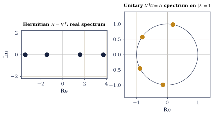
Fig. 512 The two operator classes, side by side in the complex plane. Left: a Hermitian operator’s eigenvalues (ink) lie on the real axis — they are real, and they are the possible outcomes of measuring the observable. Right: a unitary operator’s eigenvalues (amber) lie on the unit circle \(|\lambda|=1\) (grey) — the operator moves states around without changing their length, and so conserves probability. This single picture is the geometric heart of the volume: what we measure is Hermitian (real), and how states evolve is unitary (norm-preserving).

Exercise 6 — From Hermitian to unitary: the exponential map

The two classes of operator are linked by the exponential. For any Hermitian \(H\), the operator \(U=e^{-iH}\) is unitary, and its eigenvalues are \(e^{-i\lambda_j}\) where the \(\lambda_j\) are the real eigenvalues of \(H\) — the real spectrum of \(H\) carried onto the unit circle Eq. 499. This is the seed of dynamics: a Hermitian observable (energy, the Hamiltonian) generates a unitary (time evolution) through this map, \(U(t)=e^{-iHt/\hbar}\) (§6.7). The Hermitian \(H\) below is the one from Exercise 3, whose eigenvalues are already computed.

1. Compute the matrix exponential \(U=e^{-iH}\) with scipy.linalg.expm(-1j * H) (the matrix exponential — not numpy.exp, which would act element-by-element).

2. Verify \(U\) is unitary with the is_unitary helper.

3. Confirm the spectrum maps as claimed: compare the sorted eigenvalues of \(U\) (numpy.linalg.eigvals) against \(e^{-i\lambda_j}\) formed from \(H\)’s eigenvalues with numpy.exp(-1j * eigenvalues).

U = e^(−iH):  is_unitary(U) ?  True
eigenvalues(U) = e^(−iλ) ?  True
  |eigenvalues(U)| = [1. 1. 1. 1.]  (all on the unit circle)

Validation 6

✓  the exponential map U = e^(−iH) sends a Hermitian operator to a unitary one, with eigenvalues e^(−iλ) — observables generate dynamics

True

Exercise 7 — Commuting operators share an eigenbasis

Two commuting Hermitian operators are simultaneously diagonalizable: \([A,B]=0\) holds exactly when \(A\) and \(B\) share a common orthonormal eigenbasis Eq. 500 (Sakurai & Napolitano, §1.4, supply the proof). A convenient specimen is any polynomial in \(H\), which commutes with \(H\) by construction — so \(B=H^2+2H\), built from the Hermitian \(H\) of Exercise 3, must be diagonal in \(H\)’s eigenbasis. This is the statement that commuting observables are compatible, simultaneously definite, where non-commuting ones instead obey an uncertainty relation (§6.6).

1. Build \(B=H@H+2H\) — a polynomial in \(H\) — and confirm it is Hermitian with is_hermitian.

2. Verify the operators commute by checking the commutator(H, B) is the zero matrix (numpy.allclose(commutator(H, B), 0)).

3. Transform \(B\) into \(H\)’s eigenbasis with adjoint(V) @ B @ V (the adjoint you wrote in Exercise 2), and confirm the result is diagonal — its off-diagonal part (the matrix minus its diagonal, numpy.diag(numpy.diag(...))) vanishes — so the same eigenvectors diagonalize both.

is_hermitian(B) ?  True
[H, B] = 0 ?  True   (‖[H,B]‖ = 1.3e-14)
B in H's eigenbasis is diagonal ?  off-diagonal max = 9.6e-15

Validation 7

✓  commuting Hermitian operators share an eigenbasis ([H,B]=0 and B is diagonal in H's eigenbasis) — compatible observables   [max|Δ| = 1.30691e-14 (rtol=1e-06, atol=1e-10)]

True

Exercise 8 — The Pauli matrices as the canonical Hermitian operators

The three Pauli matrices \(\sigma_x,\sigma_y,\sigma_z\), given in the Setup as SX, SY, SZ, are the canonical Hermitian operators: each is Hermitian with eigenvalues \(\pm1\) and squares to the identity, \(\sigma^2=I\) Eq. 496. They also fail to commute, and they do so in a closed way — the commutator of two of them is a multiple of the third, \([\sigma_x,\sigma_y]=2i\sigma_z\) Eq. 500. These are the spin observables of Movement I, and this non-commutation is the source of the uncertainty between spin components (§6.6).

1. Take the three matrices SX, SY, SZ from the setup.

2. For each, confirm Hermiticity with is_hermitian, compute its eigenvalues with numpy.linalg.eigvalsh (the eigenvalue-only routine for Hermitian matrices) and confirm they are \(\pm1\), and check \(\sigma^2=I\) with SX @ SX and numpy.allclose.

3. Compute the commutator with the commutator helper and confirm commutator(SX, SY) equals `2j

   • SZ (numpy.allclose`).

σx: Hermitian True, eigenvalues [-1.  1.], σ² = I True
σy: Hermitian True, eigenvalues [-1.  1.], σ² = I True
σz: Hermitian True, eigenvalues [-1.  1.], σ² = I True
[σx, σy] = 2iσz ?  True   (so σx and σy do not commute)

Validation 8

✓  the Pauli matrices are Hermitian with eigenvalues ±1 and σ²=I, and [σx,σy]=2iσz — their non-commutation foreshadows incompatible observables

True

Exercise 9 — The actors on the stage (synthesis)

We now have the actors. Operators are what act on states, and in a basis they are matrices, so every question about them is a matrix computation. Two classes carry the physics. Hermitian operators, \(A=A^{\dagger}\), have real spectra and orthonormal eigenbases — they are the observables, their eigenvalues the possible measurements and their eigenvectors the definite-value states. Unitary operators, \(U^{\dagger}U=I\), preserve the inner product and hence probabilities — they are the symmetries and the dynamics. The exponential map \(U=e^{-iH}\) ties the two together, and is the seed of the statement that energy generates time. And the spectral theorem, \(A=V\Lambda V^{\dagger}\) — diagonalize, and the operator becomes transparent — is the one computation we will run again and again, from the qubit to the hydrogen atom.

There is no new computation to run here: the machinery itself is the result. Two facts will carry the entire volume, and we have now established both. Observables are Hermitian, so what we measure is real; evolution is unitary, so probability is conserved. Everything else — the postulates, uncertainty, dynamics, the spectra of real systems — is diagonalization on the space of §6.1. The next notebook (§6.3) gives all of this its proper language, Dirac notation, where the spectral theorem becomes a sum of projectors \(A=\sum_\lambda\lambda\,|\lambda\rangle\langle\lambda|\) and operators acquire their cleanest form.

Notebook summary

The actors on the Hilbert-space stage: linear operators, and the two classes that run quantum mechanics.

• Operators are matrices Eq. 494: \(A_{ij}=\langle e_i|A|e_j\rangle\), acting by @ and composing by @; in general \(AB\ne BA\).

• The adjoint Eq. 495: \(A^{\dagger}=\)A.conj().T, defined by \(\langle u|A^{\dagger}v \rangle=\langle Au|v\rangle\), with \((AB)^{\dagger}=B^{\dagger}A^{\dagger}\).

• Hermitian operators are the observables Eq. 496: \(A=A^{\dagger}\) forces real eigenvalues and an orthonormal eigenbasis (both proved); numpy.linalg.eigh is the tool.

• The spectral theorem Eq. 497: \(A=V\Lambda V^{\dagger}\) to machine precision — to understand a Hermitian operator, diagonalize it. (Projector form: §6.3.)

• Unitary operators are the symmetries and dynamics Eq. 498: \(U^{\dagger}U=I\) preserves inner products, norms, and probabilities; eigenvalues on the unit circle.

• The exponential map Eq. 499: \(U=e^{-iH}\) (via scipy.linalg.expm) is unitary for Hermitian \(H\), eigenvalues \(e^{-i\lambda}\) — energy generates evolution (§6.7).

• Commuting operators share an eigenbasis Eq. 500: \([A,B]=0\) means compatible, simultaneously definite observables; the Pauli matrices, with \([\sigma_x,\sigma_y]=2i\sigma_z\), are the canonical non-commuting example.

Two facts carry the volume: observables are Hermitian, so what we measure is real; evolution is unitary, so probability is conserved. Everything else is diagonalization.

Outlook

• Dirac notation made formal (§6.3). The spectral theorem as a sum of projectors \(A=\sum_\lambda \lambda\,|\lambda\rangle\langle\lambda|\), the resolution of the identity, and functions of operators \(f(A)=\sum_\lambda f(\lambda)\,|\lambda\rangle\langle\lambda|\).

• The measurement postulate (§6.5). Eigenvalues as outcomes, \(|\langle\lambda|\psi\rangle|^2\) as probabilities, projectors as the measurement.

• Commutators and uncertainty (§6.6). Where non-commuting observables — the Pauli matrices among them — give the uncertainty relation, grown from the Cauchy–Schwarz inequality of §6.1.

• Time evolution (§6.7). The unitary generated by the Hamiltonian, \(U(t)=e^{-iHt/\hbar}\).

• Cross-reference §6.1 (the inner-product space), §0.4–§0.5 (eigenvalue problems), and forward to §6.3, §6.5, §6.6, §6.7.

Take this notebook with you

Use the download button (↓) in the toolbar above to save this notebook and run it yourself. The published notebooks ship without worked solutions; if you would like the reference solutions — to teach from or to check your own work — get in touch: hello@ramador.me.