


6.24 Time-Dependent Perturbation Theory and Fermi’s Golden Rule#
Notebook overview#
Notebook §6.21 asked how a static perturbation shifts the energy levels. This one asks the complementary and more dynamical question: how does a perturbation that switches on drive transitions between states? Once \(H\) depends on time the energy eigenstates of \(H_0\) are no longer stationary — probability flows between them — and the object of interest is the transition probability \(P_{i\to f}(t)=|c_f(t)|^2\).
First-order time-dependent perturbation theory gives a strikingly clean answer: the amplitude to hop from \(|i\rangle\) to \(|f\rangle\) is the Fourier transform of the perturbation’s matrix element at the transition frequency \(\omega_{fi}= (E_f-E_i)/\hbar\). A perturbation oscillating at frequency \(\omega\) drives the transition only near resonance, \(\hbar\omega\approx E_f-E_i\), with a \(\mathrm{sinc}^2\) lineshape that narrows as the perturbation acts longer — energy conservation emerging dynamically. For a single discrete final state the probability oscillates (the short-time face of the Rabi problem of §6.7); but when the final states form a continuum, summing the \(\mathrm{sinc}^2\) over their density \(\rho(E)\) turns the oscillation into a probability linear in time — a constant rate. That is Fermi’s golden rule, \(\Gamma_{i\to f}=(2\pi/\hbar)|\langle f|V|i\rangle|^2\rho(E_f)\), one of the most used formulas in physics. The crossover from reversible oscillation to irreversible steady decay, as the destination goes from one level to a continuum, is the same emergence of irreversibility from reversible dynamics we met in Volume V (§5.11).
Applied to an atom in an oscillating electric field, the perturbation is the electric-dipole coupling and the matrix element is \(\langle f|\mathbf r|i \rangle\). Its angular part — an integral of three spherical harmonics — vanishes unless \(\Delta l=\pm1\) and \(\Delta m=0,\pm1\): the selection rules, which we compute directly from the hydrogen orbitals (§6.15, §6.17) rather than invoking group theory. These are why spectral lines appear where they do, and why some are missing. We keep the treatment semiclassical (classical field, quantized atom); spontaneous emission, the quantized field, and the Einstein \(A/B\) coefficients are named as Volume VII horizons, not developed here.
Method specificity. The first-order amplitude is a time integral by
scipy.integrate.quad; the continuum sum over final states isnumpy.trapezoidagainst a density of states; the dipole angular integrals usescipy.special.sph_harm_y. Selection rules are classified with a clean tolerance (\(10^{-3}\)): on this uniform grid the trapezoid rule leaves a truly forbidden integral at machine precision (\(\sim10^{-16}\)), far below the allowed values, so the threshold separates them with enormous margin.
How to read the checks. A ✗ is a prompt to locate a discrepancy — an error, a convention, or too tight a tolerance — not a verdict that the physics is wrong. Passing is strong evidence, not proof.
Theory in brief#
The time-dependent problem#
With \(H=H_0+V(t)\), expand the state in the (known) eigenstates of \(H_0\), \(|\psi(t)\rangle=\sum_n c_n(t)\,e^{-iE_n t/\hbar}|n\rangle\). The perturbation makes the coefficients evolve, so probability flows between the levels; the transition probability is
First-order transition amplitude#
To first order in \(V\), starting in \(|i\rangle\) (\(c_i\approx1\)), integrating the Schrödinger equation for the coefficients gives
The amplitude is the Fourier transform of the matrix element at the transition frequency: a transition is driven only if \(V(t)\) contains the frequency \(\omega_{fi}\).
Harmonic perturbation and resonance#
For \(V(t)=V_0\cos(\omega t)\) switched on for a time \(T\), Eq. 624 is sharply peaked when \(\omega\approx\omega_{fi}\) (absorption) or \(\omega\approx-\omega_{fi}\) (stimulated emission). Near resonance the probability is
with \(\mathrm{sinc}(x)=\sin(x)/x\). The lineshape narrows as \(\sim2\pi/T\): the longer the perturbation acts, the more sharply it enforces energy conservation \(\hbar\omega=E_f-E_i\), becoming a delta function \(\delta(E_f-E_i\mp\hbar\omega)\) as \(T\to\infty\).
Discrete versus continuum#
For a single discrete final state, \(P(T)\) near resonance grows as \(T^2\) and then oscillates — the short-time face of the Rabi problem (§6.7), and first-order theory holds only while \(P\) stays small.
When the final states form a continuum of density \(\rho(E)\), summing the \(\mathrm{sinc}^2\) over final energies (using \(\int\mathrm{sinc}^2(xT/2)\,\mathrm dx=2\pi/T\)) turns the \(T^2\) peak into a probability linear in \(T\) — a constant rate. This crossover from reversible oscillation to irreversible steady decay is the conceptual heart (echoing §5.11).
Fermi’s golden rule#
The transition rate into a continuum is therefore
evaluated at the final states that conserve energy. The coupling squared times the density of available final states: it governs decay, scattering, absorption and emission — anywhere a discrete state couples to a continuum.
Absorption, emission, and selection rules#
For an atom in a field \(\mathbf E\cos(\omega t)\) the perturbation is the electric-dipole coupling
so the matrix element is the dipole moment \(\langle f|\mathbf r|i\rangle\). Because the components of \(\mathbf r\) are proportional to the \(Y_1^\mu\), the angular part of the matrix element is an integral of three spherical harmonics, and it
with \(\mu=0\) for \(z\)-polarized light and \(\mu=\pm1\) for \(x,y\)-polarization. The photon carries one unit of angular momentum, so \(l\) must change by one and \(m\) by at most one. These are the selection rules, computed here by direct integration.
Reference: Sakurai & Napolitano (§5.6–5.7) and Griffiths [GS18] (time-dependent PT, the golden rule, atom–radiation interaction, selection rules); Nolting [Nol17]. Cross-reference §6.21 (time-independent PT), §6.7 (Rabi oscillations, the discrete two-level case), §6.15 (spherical harmonics), §6.17 (hydrogen orbitals), §5.11 (irreversibility from reversible dynamics), and forward to §6.25 (Movement VI) and Volume VII (the quantized field, spontaneous emission, Einstein coefficients — horizons).
Setup#
The data are the working units — \(\hbar=1\), the perturbation switched on at \(t=0\) and acting for a time \(T\), and unless stated a constant coupling \(V_{0,fi}=g\) — together with the tolerance that separates an allowed dipole integral from a forbidden one. The one instrument is the spherical quadrature mesh: a \((\theta,\varphi)\) grid and its \(\sin\theta\) measure, precomputed once because every angular integral in the notebook uses the same one. Building a mesh is plumbing shared by any integral over the sphere; the physics lives in the integrand.
The five objects the notebook is named for are deliberately absent: you build the first-order amplitude in Exercise 1, the \(\mathrm{sinc}^2\) lineshape in Exercise 2, the continuum sum and the golden-rule rate in Exercise 4, and the dipole angular integral in Exercise 6.
The Setup below holds this notebook’s data and instruments — nothing you are asked to build. It is collapsed so the building stays yours; expand it whenever you want the details.
Exercise 1 — The first-order transition amplitude#
Expanding the state in the eigenstates of \(H_0\) and integrating the Schrödinger equation for the coefficients to first order in \(V\) gives Eq. 624: the amplitude to arrive in \(|f\rangle\) is \(c_f=-\tfrac{i}{\hbar}\int_0^T\langle f|V(t')|i \rangle\,e^{i\omega_{fi}t'}\,\mathrm dt'\), the Fourier transform of the matrix element at the transition frequency \(\omega_{fi}\). Two consequences are visible numerically. For a constant coupling \(V_{fi}=g\) switched on at \(t=0\) the integral has the closed form \(|c_f|^2=g^2T^2\,\mathrm{sinc}^2(\omega_{fi}T/2)\), which is what the quadrature must reproduce. And the running amplitude \(\big|\int_0^t e^{i\omega_{fi}t'}\,\mathrm dt'\big|\) separates two regimes: on resonance (\(\omega_{fi}=0\)) the integrand keeps a constant phase and the amplitude grows linearly without bound, while off resonance the rotating phase makes successive contributions cancel and the amplitude merely oscillates below \(2/|\omega_{fi}|\). A perturbation drives a transition only if it contains the transition frequency — the seed of both resonance and energy conservation.
Write
first_order_amplitude(V_of_t, w_fi, T)for Eq. 624.scipy.integrate.quadintegrates real functions, so split the oscillatory integrand into its real (\(\cos\omega_{fi}t'\)) and imaginary (\(\sin\omega_{fi}t'\)) parts, quadrature each, and recombine them with the \(-i/\hbar\) prefactor. Write this one yourself — the implementation is the lesson.Evaluate it for a constant coupling \(V_{fi}=g\) at several pairs \((\omega_{fi},T)\).
Compare \(|c_f|^2\) to the closed form \(g^2T^2\,\mathrm{sinc}^2(\omega_{fi}T/2)\).
Plot the running amplitude magnitude for the resonant and off-resonant cases, with the bound \(2/|\omega_{fi}|\) marked.
w_fi=0.5, T=10.0:  |c_f|² (quad) = 5.73070   closed form = 5.73070
w_fi=1.3, T=7.0:  |c_f|² (quad) = 2.30500   closed form = 2.30500
w_fi=2.0, T=4.0:  |c_f|² (quad) = 0.57275   closed form = 0.57275
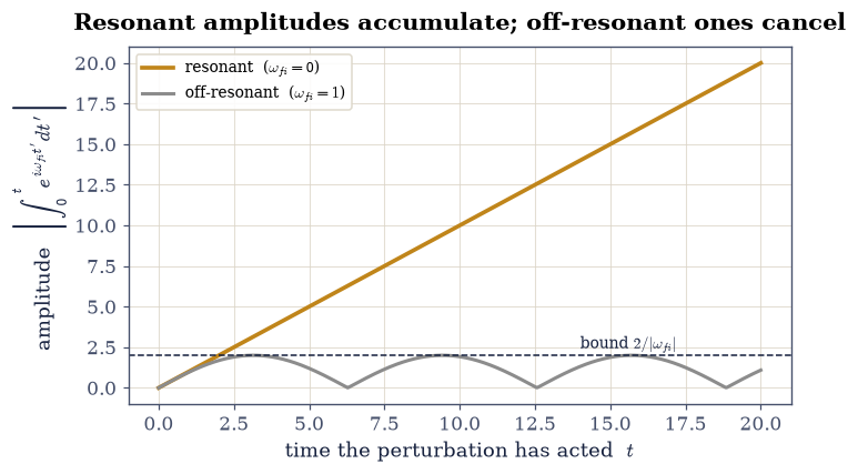
Fig. 585 Why transitions need resonance. The first-order amplitude is \(c_f\propto\int_0^t e^{i\omega_{fi}t'}\mathrm dt'\), the Fourier transform of the perturbation at the transition frequency. On resonance (\(\omega_{fi}=0\), amber) the integrand is a constant phase and the amplitude grows linearly with time; off resonance (grey) the rotating phase makes successive contributions cancel, so the amplitude merely oscillates within a bound \(2/|\omega_{fi}|\). A perturbation drives a transition only if it contains the transition frequency — the seed of both resonance and energy conservation.#
Validation 1#
The quadrature amplitude must reproduce the closed-form first-order probability \(g^2T^2\,\mathrm{sinc}^2(\omega_{fi}T/2)\): the transition amplitude is the Fourier transform of \(\langle f|V|i\rangle\) at \(\omega_{fi}\).
✓ the first-order transition probability from the quad time-integral equals g²T²·sinc²(ω_fi T/2) (the amplitude is the Fourier transform of ⟨f|V|i⟩)
True
Exercise 2 — Resonance and the sinc² lineshape#
A harmonic perturbation \(V_0\cos(\omega t)\) acting for a time \(T\) gives the near-resonant
probability Eq. 625, whose frequency dependence is the factor
\(\mathrm{sinc}^2[(\omega-\omega_{fi})T/2]\): a peak centred on \(\omega=\omega_{fi}\), which
is the energy-conservation condition \(\hbar\omega=E_f-E_i\) wearing the shape of a
spectral line. Its width is what repays measuring. The first zeros of the factor sit
at \((\omega-\omega_{fi})T/2=\pm\pi\), so the peak narrows as \(\sim2\pi/T\) and the product
\(T\cdot\text{FWHM}\) should come out constant — the longer the perturbation acts, the
more sharply it enforces energy conservation, until as \(T\to\infty\) the lineshape
becomes a delta function. Extracted from the sampled curve rather than assumed, that
constant is the energy–time uncertainty relation as a measurement. One implementation
trap: numpy.sinc is the normalized sinc, \(\sin(\pi x)/(\pi x)\), so its argument
must be divided by \(\pi\).
Write
sinc2_lineshape(w, w_fi, T)for the resonance factor of Eq. 625, and evaluate it over a range of drive frequencies \(\omega\).Confirm the peak sits at \(\omega=\omega_{fi}\).
Measure the full width at half maximum from the half-maximum crossings of the sampled curve, at four durations \(T\).
Confirm the width scales as \(1/T\) — that the product \(T\cdot\text{FWHM}\) is constant.
Cite Eq. 625.
peak of the lineshape at ω = 4.999  (ω_fi = 5.0)
  T=  5.0:  FWHM = 1.1118   T·FWHM = 5.559
  T= 10.0:  FWHM = 0.5536   T·FWHM = 5.536
  T= 20.0:  FWHM = 0.2776   T·FWHM = 5.551
  T= 40.0:  FWHM = 0.1365   T·FWHM = 5.461
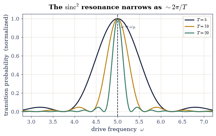
Fig. 586 Energy conservation emerging in time. The transition probability for a harmonic perturbation is a \(\mathrm{sinc}^2\) in the detuning \(\omega-\omega_{fi}\), peaked at resonance \(\omega=\omega_{fi}\) (dashed) where \(\hbar\omega=E_f-E_i\). As the perturbation acts longer the peak grows and narrows — its width scales as \(2\pi/T\) — so the longer one waits, the more sharply only energy-conserving transitions survive. In the limit \(T\to\infty\) the lineshape becomes a delta function: exact energy conservation, produced dynamically.#
Validation 2#
The lineshape must peak at \(\omega_{fi}\) and its width must scale as \(1/T\), i.e. the product \(T\cdot\text{FWHM}\) is (nearly) constant across durations.
✓ P(ω) peaks at ω_fi with a sinc² lineshape whose FWHM scales as 1/T (T·FWHM constant): resonant transitions conserve energy
True
Exercise 3 — A discrete final state: the short-time Rabi connection#
For a single resonant final state, first-order theory gives \(P_1(t)=(\Omega t/2)^2\) with the Rabi frequency \(\Omega=|V_{0,fi}|/\hbar\) — and §6.7 has already solved the very same two-level problem exactly, \(P(t)=\sin^2(\Omega t/2)\). The first is the small-angle expansion of the second, so the two must agree while \(\Omega t\ll1\) and part company as the population cycles. Where they part is where the approximation announces its own expiry: the first-order parabola climbs past \(P=1\), which no probability may do, while the exact result turns over and oscillates back. Perturbation theory is trustworthy only while \(P\) stays small, and a discrete transition is reversible — probability sloshes between the two levels instead of draining away, which is exactly the behaviour the continuum of Exercise 4 will destroy.
Evaluate the first-order \(P_1(t)=(\Omega t/2)^2\) and the exact \(P(t)=\sin^2(\Omega t/2)\) on a common time grid.
Confirm they agree at short time, on the mask \(\Omega t<0.4\).
Locate the time at which \(P_1\) first exceeds 1 — beyond it the exact treatment of §6.7 takes over.
Overlay the two curves with \(P=1\) marked.
Cite Eq. 626.
short time (Ωt<0.4): max|P₁ − sin²| = 4.94e-04
first-order P exceeds 1 at Ωt = 2.01 (PT has broken down; exact Rabi stays ≤ 1)
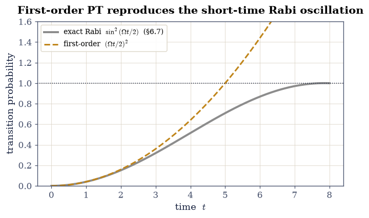
Fig. 587 First-order theory is the short-time face of Rabi. For a single resonant final state the first-order probability \((\Omega t/2)^2\) (amber) is exactly the leading term of the exact two-level Rabi oscillation \(\sin^2(\Omega t/2)\) (grey, §6.7): the two agree while \(\Omega t\ll1\). But first-order theory knows nothing of saturation — its parabola climbs past 1 (dashed) — whereas the exact probability turns over and oscillates back. Perturbation theory is trustworthy only while the transition probability stays small; a discrete transition is reversible, sloshing between the two levels.#
Validation 3#
At short time first-order theory and the exact Rabi oscillation must coincide: \((\Omega t/2)^2\approx\sin^2(\Omega t/2)\) for \(\Omega t\ll1\).
✓ first-order PT matches the short-time Rabi oscillation sin²(Ωt/2) (§6.7) [max|Δ| = 0.000494329 (rtol=0.01, atol=0.001)]
True
Exercise 4 — Fermi’s golden rule: a rate into a continuum#
Now change the destination from one level to many. Take a band of final states of density \(\rho\) (states per unit energy) around resonance, each coupled by the same \(g\), and add up their first-order probabilities: \(P(T)=\int\rho(E)\,|c_f(T)|^2\,\mathrm dE\) with \(|c_f|^2=g^2T^2\,\mathrm{sinc}^2(\omega_{fi}T/2)\) Eq. 626. The \(T^2\) out front looks like the discrete case, but the \(\mathrm{sinc}^2\) narrows as \(1/T\) while it grows, and \(\int\mathrm{sinc}^2(xT/2)\,\mathrm dx=2\pi/T\) converts one factor of \(T\) into a constant. What survives is a probability linear in \(T\) — a constant rate — and that rate is Fermi’s golden rule \(\Gamma=(2\pi/\hbar)|g|^2\rho\) Eq. 627. The contrast to keep in view is a single, slightly detuned discrete state, for which \(P(T)=g^2\,4\sin^2(\delta T/2)/ \delta^2\) merely oscillates: the same coupling drains irreversibly into a continuum and sloshes reversibly into a level. The crossover is where irreversibility enters, and it arrives from the number of places to go, not from any dissipation put in by hand.
Write
continuum_probability(T, rho, band, g): form \(g^2T^2\,\mathrm{sinc}^2 (\omega_{fi}T/2)\) over a band of final energies and integrate it against \(\rho\) withnumpy.trapezoid.Write
golden_rule_rate(V_fi, rho)for \(\Gamma=(2\pi/\hbar)|V_{fi}|^2\rho\) Eq. 627.Show \(P(T)\) grows linearly in \(T\) (so \(P/T\) is constant), and that \(P/T\) agrees with \(\Gamma\).
Contrast on one plot with the single detuned discrete state.
  T=  20.0:  P=1.24676e-02   P/T=6.23380e-04
  T=  40.0:  P=2.50326e-02   P/T=6.25815e-04
  T=  80.0:  P=5.01656e-02   P/T=6.27070e-04
  T= 160.0:  P=1.00431e-01   P/T=6.27694e-04
  T= 320.0:  P=2.00962e-01   P/T=6.28006e-04
golden rule Γ = (2π/ℏ)|g|²ρ = 6.28319e-04   (numeric P/T → this)
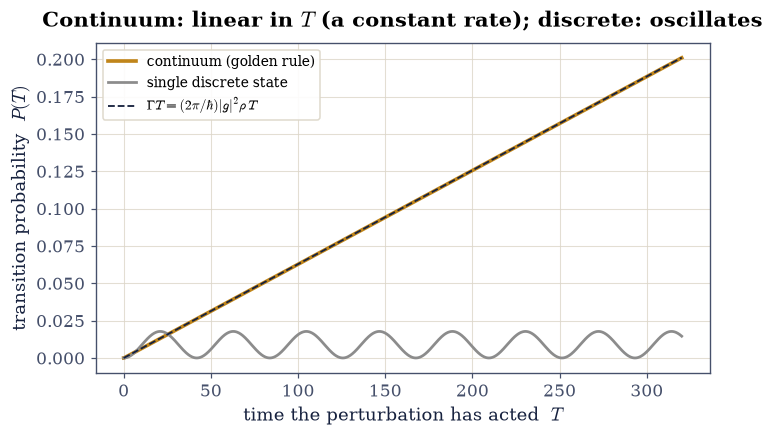
Fig. 588 Reversible oscillation becomes irreversible decay. Into a single (slightly detuned) discrete state the probability merely oscillates (grey) — the flow is reversible, sloshing back and forth, as for Rabi. But summed over a continuum of final states, the \(\mathrm{sinc}^2\) peaks add up to a probability that grows linearly in time (amber): a constant rate. That rate is Fermi’s golden rule \(\Gamma=(2\pi/\hbar)|g|^2\rho\) (the numeric slope matches it). The crossover from oscillating to steadily draining, as the destination goes from one level to many, is where irreversibility enters — the same theme as Volume V (§5.11).#
Validation 4#
Into a continuum the probability must be linear in time — a constant rate — equal to Fermi’s golden rule \(\Gamma=(2\pi/\hbar)|g|^2\rho\). We check \(P/T\) is constant across durations and matches the formula.
✓ the continuum transition probability is linear in time — a constant rate Γ=(2π/ℏ)|g|²ρ (Fermi's golden rule) [got 0.000628006 vs expected 0.000628319 (rtol=0.02, atol=1e-09)]
True
Exercise 5 — Absorption and emission of light#
Put an atom in a field \(\mathbf E\cos(\omega t)\) and the perturbation is the electric-dipole coupling \(V(t)=-e\,\mathbf E\cdot\mathbf r\,\cos(\omega t)\) Eq. 628, so the matrix element the golden rule asks for is the dipole moment \(\langle f|\mathbf r|i\rangle\). The \(\cos(\omega t)\) carries two resonances Eq. 625, one for each sign of \(\omega_{fi}\): at \(\hbar\omega=E_f-E_i>0\) the atom climbs and takes a quantum from the field — absorption; at \(E_f<E_i\) it falls and adds one — stimulated emission. Both rates are proportional to the same \(|\langle f|\mathbf r|i\rangle|^2\), which is why Einstein’s two \(B\) coefficients are equal, and it means a vanishing dipole moment leaves no first-order line at all — the opening that Exercises 6 and 7 walk through. Spontaneous emission, decay with no applied field, is absent from this semiclassical picture: it requires quantizing the field, and with it comes the Einstein \(A/B\) relation (Volume VII horizon).
Draw the two resonances as mirror level diagrams — the same matrix element, the arrows reversed.
Confirm with the
golden_rule_rateyou wrote in Exercise 4 that the rate scales as \(|\langle f|\mathbf r|i\rangle|^2\).
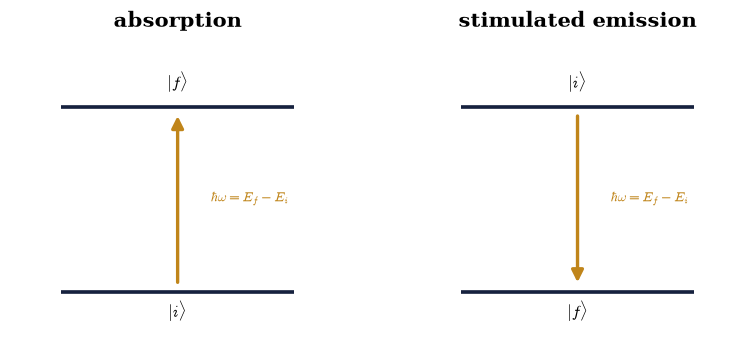
Fig. 589 The two faces of a resonant transition. When the photon energy \(\hbar\omega\) matches a level spacing \(E_f-E_i\), the oscillating field drives the atom between the levels through its dipole moment \(\langle f|\mathbf r|i\rangle\): absorption (left) takes the atom up and removes a quantum from the field; stimulated emission (right) takes it down and adds one. The golden rule gives both rates, equal and proportional to \(|\langle f|\mathbf r|i\rangle|^2\). Spontaneous emission — decay with no field present — is absent from this semiclassical picture and requires quantizing the field (Volume VII).#
Validation 5#
The absorption and stimulated-emission rates are set by the same dipole matrix element through the golden rule; a nonzero dipole moment gives a finite rate. We check the golden-rule rate scales as \(|\langle f|\mathbf r|i\rangle|^2\).
✓ the absorption/emission rate scales as |⟨f|r|i⟩|² via the golden rule (light absorption and emission are dipole transitions at resonance)
True
Exercise 6 — Selection rules from the hydrogen orbitals#
The components of \(\mathbf r\) are proportional to the \(Y_1^\mu\) — \(\mu=0\) for
\(z\)-polarized light, \(\mu=\pm1\) for \(x,y\) — so the angular part of the dipole matrix
element between \(|l,m\rangle\) and \(|l',m'\rangle\) is an integral of three spherical
harmonics, \(\int Y_{l'm'}^{*}Y_1^{\mu}Y_{lm}\,\mathrm d\Omega\)
Eq. 629. The claim to be tested is that it vanishes unless \(\Delta
l=\pm1\) and \(\Delta m=\mu\): the photon carries one unit of angular momentum, so \(l\)
must change by one and \(m\) by at most one. Group theory settles this in a line; here it
emerges from doing the integrals, over the states \(l=0,1,2\) on the \((\theta,\varphi)\)
grid the Setup precomputed. The verdict is unambiguous because the numbers are — a
forbidden integral comes out at machine precision (\(\sim10^{-16}\)) and an allowed one
at order \(10^{-1}\), so the threshold SEL_TOL \(=10^{-3}\) separates the two with
thirteen decades to spare.
Write
dipole_angular_integral(lp, mp, l, m, mu)for Eq. 629: evaluate the three harmonics on the Setup grid withscipy.special.sph_harm_y, include the \(\sin\theta\) measure, and integrate over \(\varphi\) and then \(\theta\) withnumpy.trapezoid.Evaluate it for every pair \((l',m')\leftarrow(l,m)\) with \(l,l'\le2\), keeping the largest value over the polarizations \(\mu\in\{-1,0,1\}\).
Classify each pair as allowed or forbidden at the tolerance
SEL_TOL.Read off the pattern: nonzero only for \(\Delta l=\pm1\), and \(\Delta m=\mu\).
Cite Eq. 629.
allowed transitions all satisfy Δl=±1 and |Δm|≤1: True
example: |1,0⟩→|2,0⟩ (z, Δl=+1,Δm=0) = 0.2523
example: |1,0⟩→|0,0⟩ (Δl=−1,Δm=0)    = 0.2821
forbidden: |0,0⟩→|0,0⟩ (Δl=0)        = 1.39e-17
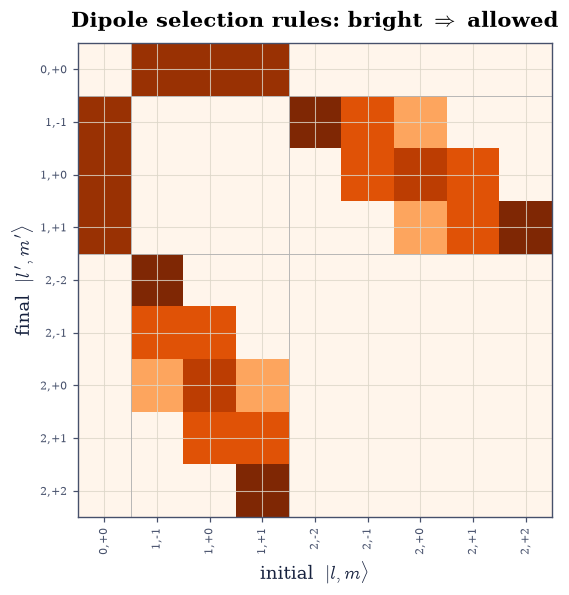
Fig. 590 The selection rules, computed not asserted. Each cell is the dipole angular integral \(\big|\int Y_{l'm'}^{*}Y_1^{\mu}Y_{lm}\,\mathrm d\Omega\big|\) (maximized over polarization \(\mu\)) connecting an initial state \(|l,m\rangle\) (columns) to a final state \(|l',m'\rangle\) (rows); amber is allowed, blank is forbidden. The bright entries fall exactly on \(\Delta l=\pm1\) with \(\Delta m=0,\pm1\) — every other transition vanishes. The photon carries one unit of angular momentum, so \(l\) must change by one and \(m\) by at most one; the whole of dipole spectroscopy is in this pattern, and we obtained it by doing the integrals.#
Validation 6#
Every allowed dipole transition must satisfy \(\Delta l=\pm1\) and \(\Delta m=0,\pm1\), and no others: the selection rules follow from the spherical-harmonic integrals.
✓ the dipole angular integrals are nonzero only for Δl=±1 and Δm=0,±1 (the selection rules follow from the Y-integrals, not group theory)
True
Exercise 7 — A forbidden transition, and why lines are missing (student)#
Selection rules are not bookkeeping: they decide which spectral lines an atom can emit, and which states get stranded. Hydrogen’s \(2s\) is the textbook casualty. The decay \(2s\to1s\) takes \(l=0\) to \(l'=0\), so \(\Delta l=0\) and the dipole rule forbids it, while its neighbour \(2p\to1s\) has \(\Delta l=-1\) and is allowed. With the direct electric-dipole channel closed, the \(2s\) state cannot shed its energy the fast way and becomes metastable, decaying only through far slower higher-order and multipole processes — which is exactly why some expected spectral lines come out faint, or missing altogether.
Compute the \(2s\to1s\) angular integral for every polarization \(\mu\) with the
dipole_angular_integralyou wrote in Exercise 6, and show all three vanish.Compute the \(2p\to1s\) set the same way and show it contains nonzero entries.
Draw the two channels on one level diagram, the allowed beside the forbidden.
2s→1s (Δl=0) dipole integrals, all μ: ['9.61e-18', '1.39e-17', '9.61e-18']  → forbidden
2p→1s (Δl=−1) largest dipole integral: 0.2821  → allowed
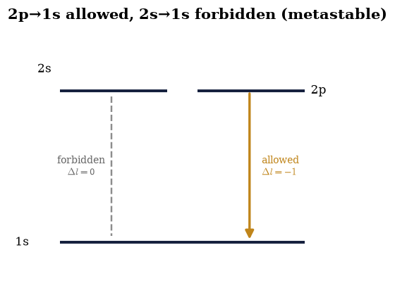
Fig. 591 Why the \(2s\) state lives so long. The \(2p\to1s\) transition (amber) has \(\Delta l=-1\) and is dipole-allowed, so it is fast — an ordinary bright line. The \(2s\to1s\) transition (grey, dashed) has \(\Delta l=0\); its dipole matrix element vanishes identically, so the direct electric-dipole decay is forbidden. The \(2s\) state cannot shed its energy this way and becomes metastable, decaying only through far slower higher-order processes. Selection rules are not bookkeeping: they decide which spectral lines an atom can emit, and which states get stranded.#
Validation 7#
A \(\Delta l=0\) transition (\(2s\to1s\)) must have a vanishing dipole matrix element for every polarization — forbidden — while the \(\Delta l=\pm1\) neighbor (\(2p\to1s\)) does not.
✓ a Δl=0 transition (2s→1s) has vanishing dipole matrix element (forbidden), producing the metastable 2s state and missing lines
True
Exercise 8 — (Synthesis) The rule behind the spectrum#
A perturbation that changes in time sets probability flowing between states, favouring — ever more sharply the longer it acts — the transitions that conserve energy. When the destination is a single level the flow sloshes back and forth, reversible, the short-time face of Rabi. When it is a continuum, the sloshing becomes a steady drain, and its rate is Fermi’s golden rule: the coupling squared times the density of places to go. That one crossover — from oscillation to irreversible decay as one level becomes many — is the same passage from reversible microscopics to irreversible macroscopics we watched in Volume V (§5.11), here in its cleanest quantum form.
Applied to an atom in a light field, the coupling is the dipole moment, and the geometry of the spherical harmonics decides which transitions are allowed: \(\Delta l=\pm1\), one unit of angular momentum handed to the photon. This is the machinery of spectroscopy, and with it Movement V is complete. We have met the three faces of approximation — perturbative (§6.21), variational (§6.22), semiclassical (§6.23) — and now the dynamics of transitions that turns all of them toward experiment. The golden rule looks almost too simple for how much it carries: a matrix element, a density of states, a factor of \(2\pi\). Yet every glowing gas, every laser line, every fluorescent lifetime is that formula, and the reason a neon sign is orange is a set of dipole integrals we just did by hand.
The final movement returns to the foundations — to the correlations that have no classical explanation at all. The next notebook (§6.25) turns the Bell-state puzzle of Movement I into a quantitative inequality, and watches quantum mechanics violate it.
Notebook summary#
First-order amplitude Eq. 624: the transition amplitude is the Fourier transform of \(\langle f|V|i\rangle\) at \(\omega_{fi}\) (verified: the
quadtime-integral equals \(g^2T^2\,\mathrm{sinc}^2\)).Resonance Eq. 625: the \(\mathrm{sinc}^2\) lineshape peaks at \(\omega_{fi}\) and narrows as \(2\pi/T\) — energy conservation emerging in time.
Discrete vs continuum Eq. 626: first-order PT is the short-time face of Rabi (§6.7); into a continuum the probability goes linear in \(T\).
Fermi’s golden rule Eq. 627: \(\Gamma=(2\pi/\hbar)|V_{fi}|^2\rho\), the numeric continuum rate matching the formula (
numpy.trapezoidover the band).Selection rules Eq. 629: the dipole angular integrals (
scipy.special.sph_harm_y) are nonzero only for \(\Delta l=\pm1\), \(\Delta m=0,\pm1\); the \(\Delta l=0\) \(2s\to1s\) integral vanishes — the metastable \(2s\).
Outlook#
Bell’s inequality (§6.25): the Movement I entanglement puzzle made quantitative, and its quantum violation computed — opening Movement VI.
The quantized radiation field, spontaneous emission, and the Einstein \(A/B\) coefficients; natural line widths and lifetimes (Volume VII; horizons).
Scattering as a golden-rule process and the Born approximation (a horizon).
Cross-reference §6.21 (time-independent PT), §6.7 (Rabi), §6.15 (spherical harmonics), §6.17 (hydrogen orbitals), §5.11 (irreversibility), forward to §6.25 and Volume VII.