5.4 Microstates, Entropy, Temperature, and the Boltzmann Distribution

Elementary Computational Physics

Volume V — Classical Statistical Mechanics Notebook 5.4

Where counting becomes physics. From the postulate that every accessible microstate is equally likely — the microcanonical ensemble — we count our way to entropy, watch the second law emerge as a system finding its most probable state, discover what temperature actually is, and derive the Boltzmann factor that governs everything that follows.

Level · advanced   •   Est. · 160–200 min

Raymond Amador v1.4.0  ·  2026-07-31  ·  CC BY 4.0 (text) / MIT (code)

Notebook overview

This is the first physics notebook of Volume V, and it makes good on a promise the math arsenal has been building toward: that counting microstates is doing statistical mechanics. From a single postulate — every accessible microstate of an isolated system is equally likely — and the combinatorics of §5.1–§5.3, we will construct the entire conceptual core of the subject. The ensemble of equally-probable microstates of an isolated system, at fixed energy, volume, and particle number, has a name we will use throughout: the microcanonical ensemble. Entropy will turn out to be the logarithm of its multiplicity. The second law will turn out to be nothing more than a system drifting to its most probable macrostate. Temperature will emerge, not be assumed, as the energy-derivative of entropy. And the Boltzmann factor \(e^{-E/kT}\), the formula the rest of statistical mechanics runs on, will fall out of counting a reservoir’s microstates.

We make this concrete with the two-state paramagnet: \(N\) classical spins in a magnetic field, each pointing either up or down. It is a genuinely classical system — “a spin that points two ways” is an ordinary modelling assumption, needing no quantum mechanics to posit — and its multiplicity is the binomial coefficient we counted in §5.1, so every step of the argument is exact. The arsenal is everywhere here, and we flag it as we go: the multiplicity is the \(\binom{N}{N_\uparrow}\) of §5.1; we compute it in log space with scipy.special.gammaln because the counts overflow (the lesson of §5.3 and §0.1); the equilibrium peak is razor-sharp for the \(1/\sqrt N\) reason of §5.3; and entropy is the log-multiplicity we first met in §5.3. What was abstract there becomes physical here.

We will (1) meet microstates and the postulate on a tiny spin system, (2) derive the paramagnet multiplicity, (3) read entropy off it, (4) bring two paramagnets into thermal contact and find the sharp equilibrium peak, (5) watch the second law emerge as energy relaxes to that peak, (6) extract temperature as \(1/T=\partial S/\partial E\), (7) derive the Boltzmann distribution from a reservoir, and (8) push the definition to its breaking point with negative temperature.

How to read the checks. Each exercise closes with a validate call against an independent fact: macrostate probabilities equal to multiplicities; the paramagnet \(\binom{N}{N_\uparrow}\); extensive entropy maximal at half-filling; the equilibrium partition at proportional energy sharing; the total entropy maximized there; equal \(\partial S/\partial E\) defining temperature; the Boltzmann \(e^{-E/kT}\) from reservoir counting; a negative slope past half-filling. A ✓ is strong evidence; a ✗ is a prompt to locate the discrepancy, not a verdict.

Scope. The microcanonical ensemble and the conceptual core of statistical mechanics from counting; why an ensemble average over phase space is valid at all is §5.5 (ergodicity), and the canonical ensemble that systematizes the Boltzmann bridge comes later in the volume. See Schroeder, An Introduction to Thermal Physics; Kardar, Statistical Physics of Particles; and §5.1 (the binomial count), §5.3 (log space, entropy, \(1/\sqrt N\)).

Theory in brief

Microstates, macrostates, and the microcanonical ensemble

A microstate is a complete specification of a system; a macrostate is a coarse description (a total energy, a particle number) compatible with many microstates. The number of microstates realizing a macrostate is its multiplicity \(\Omega\) — the counting of §5.1, now physical. The whole subject rests on one assumption,

(398)\[\text{an isolated system in equilibrium is equally likely to be in any accessible microstate,}\]

and the collection of those equally-probable microstates of an isolated system (fixed \(E\), \(V\), \(N\)) is the microcanonical ensemble. A macrostate’s probability is then proportional to its multiplicity Eq. 399,

(399)\[P(\text{macrostate})=\frac{\Omega(\text{macrostate})}{\Omega_{\rm total}} .\]

The two-state paramagnet

Our exactly-countable model is \(N\) classical spins in a magnetic field, each up (\(\sigma=+1\), energy \(+\varepsilon\)) or down (\(\sigma=-1\), energy \(0\)). The energy is set by the number pointing up, \(E=N_\uparrow\,\varepsilon\), and the number of microstates with \(N_\uparrow\) up is the count of which spins are up — a binomial coefficient,

(400)\[\Omega(N,N_\uparrow)=\binom{N}{N_\uparrow} ,\]

exactly the combinations of §5.1. The ground state is all spins down (\(N_\uparrow=0\), one microstate); the counts overflow almost at once, so we work with \(\ln\Omega\) via scipy.special.gammaln (the §5.3 lesson).

Entropy

Boltzmann’s formula, the log-multiplicity of §5.3 made physical,

(401)\[S=k\ln\Omega ,\]

is extensive (scales with system size). For the paramagnet it is maximal at half-filling (\(N_\uparrow=N/2\), the most ways to arrange the spins) and vanishes at the extremes.

Thermal contact and the second law

Bring two paramagnets \(A\) and \(B\) into contact, free to exchange energy at fixed total \(N_\uparrow=N_\uparrow^A+N_\uparrow^B\). The total multiplicity is a product,

(402)\[\Omega_{\rm total}(N_\uparrow^A)=\Omega_A(N_\uparrow^A)\,\Omega_B(N_\uparrow-N_\uparrow^A) ,\]

and it is sharply peaked (the \(1/\sqrt N\) sharpness of §5.3) at the partition that maximizes \(S_A+S_B\). Energy flows to maximize the total multiplicity: the second law is not a separate postulate but the statement that an isolated system drifts to its most probable macrostate.

Temperature

At the peak, \(\partial S_A/\partial E_A=\partial S_B/\partial E_B\). The quantity that equalizes when energy stops flowing defines temperature,

(403)\[\frac{1}{T}=\frac{\partial S}{\partial E} .\]

A body with the smaller \(\partial S/\partial E\) (the hotter one) gives up energy.

The Boltzmann distribution

Put a small system in contact with a large reservoir at temperature \(T\). By the postulate, the probability the small system sits in a microstate of energy \(E\) is proportional to the number of reservoir microstates left, \(\Omega_{\rm res}(E_{\rm tot}-E)\). Since \(\ln\Omega_{\rm res}\) falls linearly in the energy handed over, with slope \(1/kT\),

(404)\[P(E)\propto\Omega_{\rm res}(E_{\rm tot}-E)\propto e^{-E/kT} .\]

This is the master formula of statistical mechanics, and it is a counting result.

Setup

Data and instruments only: the series palette and a spin-row drawing helper for the schematic figures. The engine of the notebook is deliberately not here — you write the paramagnet log-multiplicity ln_omega_paramagnet in Exercise 2, and every entropy curve, equilibrium peak, temperature slope and Boltzmann factor that follows is computed with it, as is the spin-exchange relaxation you write in Exercise 5.

The Setup below holds this notebook’s data and instruments — nothing you are asked to build. It is collapsed so the building stays yours; expand it whenever you want the details.

Show code cell source

Hide code cell source

from math import comb

import matplotlib.pyplot as plt
import numpy as np
from matplotlib.animation import FuncAnimation
from scipy.special import gammaln

from ecp import combinatorics as cb
from ecp import draw, validate
from ecp.animate import show

# data: the series palette
ACCENT, INK, SOFT = draw.ACCENT, draw.INK, draw.SOFT


# instrument: a drawing scaffold — laying arrow glyphs along a row is how the
# paramagnet is pictured, not something any exercise here is about.
def spin_row(ax, up_mask, x0=0.0, y=0.0, pitch=0.5):
    """Draw a row of up/down spin arrows, a schematic of a paramagnet configuration.

    Each site is an arrow pointing up (aligned, energy +ε, amber) or down
    (energy 0, ink). The arrows are inline glyphs, exempt from the collision gate.

    Parameters
    ----------
    ax : matplotlib.axes.Axes
        Axes to draw on.
    up_mask : sequence of bool
        Per-site spin direction (``True`` = up).
    x0, y : float, optional
        Lower-left position of the first spin.
    pitch : float, optional
        Horizontal spacing between spins (default ``0.5``).

    Returns
    -------
    None
        Draws the spin row onto ``ax`` in place.
    """
    for i, up in enumerate(up_mask):
        ax.text(
            x0 + i * pitch,
            y,
            r"$\uparrow$" if up else r"$\downarrow$",
            fontsize=20,
            ha="center",
            va="center",
            color=ACCENT if up else INK,
            gid="_nocheck",
        )

Exercise 1 — Microstates, macrostates, and the postulate (worked)

We start with the one idea everything rests on, on a system small enough to write out in full. Take three spins, each up or down. A microstate is a complete specification — which spin points which way — and there are \(2^3=8\) of them. A macrostate is the coarse description we actually care about, here the number of up-spins (which fixes the energy), and there are only four: \(0,1,2,3\). Each macrostate is compatible with several microstates, and the count is the multiplicity: \(1,3,3,1\). The fundamental postulate Eq. 398 says every microstate is equally likely — this is the microcanonical ensemble — so each of the eight has probability \(1/8\), and therefore a macrostate’s probability is simply its multiplicity over the total Eq. 399 (Fig. 413). The most probable macrostate is the one realised the most ways. That single sentence, scaled to \(10^{23}\), is the whole of equilibrium statistical mechanics.

Part a) Enumerate the eight microstates of three spins with itertools.product, group them by number of up-spins to get each macrostate’s multiplicity, and divide those by the total to get the macrostate probabilities the postulate demands.

Part b) Confirm the enumerated multiplicities are the binomial coefficients \(C(3,k)=1,3,3,1\) of §5.1 (math.comb) and that the probabilities really are multiplicity over total — the postulate in action.

microstates (complete spin specifications): 8
macrostates (number of up-spins):  multiplicities [1, 3, 3, 1]
macrostate probabilities = multiplicity / 8 = [0.125, 0.375, 0.375, 0.125]
the most probable macrostate (1 or 2 up) is realised the most ways

Validation 1

✓  the enumerated multiplicities are the binomial C(3,k)=1,3,3,1 and set the macrostate probabilities

True

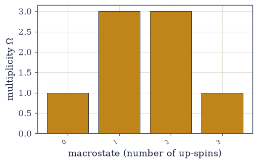
Fig. 413 The fundamental postulate on three spins. There are \(2^3=8\) equally likely microstates (complete up/down specifications) — the microcanonical ensemble — grouped into four macrostates by the number of up-spins, with multiplicities \(1,3,3,1\). Because every microstate is equally likely, a macrostate’s probability is just its multiplicity over the total, so the most probable macrostate is the one realised the most ways. Scaled to \(10^{23}\) spins, this is the entire content of equilibrium.

Exercise 2 — The paramagnet multiplicity (worked)

To do physics we need a model we can count exactly, and the two-state paramagnet is the cleanest one there is: \(N\) classical spins in a magnetic field, each pointing up or down (Fig. 414). With each up-spin carrying energy \(\varepsilon\) and each down-spin zero, a macrostate is fixed by the number of up-spins \(N_\uparrow\) (which sets the energy \(E=N_\uparrow\varepsilon\)), and its multiplicity is the number of ways to choose which \(N_\uparrow\) of the \(N\) spins are up. That is exactly the combinations count of §5.1, the binomial coefficient \(\Omega=\binom{N}{N_\uparrow}\) Eq. 400. Nothing here is quantum: a spin that points two ways is an ordinary classical modelling assumption. The numbers explode immediately — a modest magnet has a multiplicity with thousands of digits — so, exactly as §5.3 warned, we never compute \(\Omega\) itself but its logarithm, with scipy.special.gammaln. The route into log space is the factorial identity \(\binom{N}{N_\uparrow}=N!/[N_\uparrow!\, (N-N_\uparrow)!]\) read through \(\Gamma(n+1)=n!\): taking logarithms turns the quotient into a difference of three \(\ln\Gamma\) values, each of which gammaln returns directly, without ever forming the enormous factorials. Small \(N\) gives us a reference the exact integer arithmetic of math.comb can still supply, and \(N=4000\) gives us the regime where it cannot: there \(\binom{4000}{2000}\) is an integer of some \(1200\) digits, which overflows a float outright.

Part a) Write ln_omega_paramagnet(N_up, N), the log-multiplicity \(\ln\Omega(N,N_\uparrow)=\ln\binom{N}{N_\uparrow}\) Eq. 400 of the two-state paramagnet, as \(\ln\Gamma(N+1)-\ln\Gamma(N_\uparrow+1)-\ln\Gamma(N-N_\uparrow+1)\) evaluated with scipy.special.gammaln; take N_up as a float array so that a whole energy axis comes back in one call, and never form \(\Omega\) itself. Write this one yourself — the implementation is the lesson, and every entropy curve, equilibrium peak, temperature slope and Boltzmann factor in the rest of this notebook is computed with it.

Part b) Certify it against exact integer arithmetic: for \(N=10\), \(N_\uparrow=3\) compare \(\ln\Omega\) with the logarithm of math.comb(10, 3), and then show that at \(N=4000\) (half up) the exact count overflows a float while the logarithm stays finite.

paramagnet N=10 spins, N↑=3:
  Ω = C(N, N↑) = C(10,3) = 120
  ln Ω (gammaln) = 4.78749  vs  ln(120) = 4.78749

N=4000 spins (half up): Ω overflows a float (True); ln Ω = 2768.2  (finite)

Validation 2

✓  the paramagnet multiplicity is the binomial count C(N, N↑)   [got 4.78749 vs expected 4.78749 (rtol=1e-09, atol=1e-09)]
✓  the macroscopic multiplicity overflows a float; its logarithm via gammaln does not

True

Fig. 414 A two-state paramagnet. Twelve classical spins each point up (amber, energy \(\varepsilon\)) or down (ink, energy \(0\)); one configuration with five up is shown. The number of configurations with \(N_\uparrow\) up is the count of which spins are up — exactly the binomial coefficient \(\binom{N}{N_\uparrow}\) of §5.1. This single exactly-countable, genuinely classical multiplicity is the engine of the entire notebook.

Exercise 3 — Entropy as log-multiplicity (worked)

With the multiplicity in hand, entropy costs us nothing new: it is Boltzmann’s formula \(S=k\ln\Omega\) Eq. 401, the log-multiplicity of §5.3 with a name and a constant. The paramagnet’s entropy has a telling shape (Fig. 415). It vanishes at the extremes — all spins down or all up is a single microstate, \(\Omega=1\), \(S=0\) — and is maximal at half-filling \(N_\uparrow=N/2\), where there are the most ways to arrange the spins. Between, it rises and falls, the entropy of mixing of §5.3 in physical dress. And it is extensive: a magnet twice as large at the same fraction of up-spins has twice the entropy, because \(\ln\Omega\) scales with system size (a fact Stirling makes exact in the large-\(N\) limit of §5.3). Extensivity is what lets entropy, like energy, be summed over the parts of a composite system — the property we lean on in the next exercise.

Part a) Compute \(S/k=\ln\Omega(N,N_\uparrow)\) across the full energy axis of an \(N=100\) paramagnet, with the ln_omega_paramagnet you wrote in Exercise 2.

Part b) Confirm the curve is maximal at half-filling, \(S_{\max}=\ln\binom{N}{N/2}\) at \(N_\uparrow=N/2\), and vanishes at both extremes.

Part c) Test extensivity at large \(N\): evaluate \(\ln\Omega(N,N_\uparrow)\) and \(\ln\Omega(2N,2N_\uparrow)\) at the same fraction of up-spins (\(N=1000\), \(N_\uparrow=250\)) and confirm their ratio is \(2\).

paramagnet N=100:  S/k = 0 at the extremes (0.0, 0.0),
  maximal at N↑=N/2: S_max = ln C(100,50) = 66.784

extensivity (N↑/N=1/4): ln Ω(N) = 558.80,  ln Ω(2N,2N↑) = 1120.79
ratio = 2.0057  (→ 2: entropy is extensive)

Validation 3

✓  the entropy is maximal at half-filling (N↑=N/2) and vanishes at the extremes
✓  entropy is extensive — it scales with system size   [got 2.00571 vs expected 2 (rtol=0.01, atol=1e-09)]

True

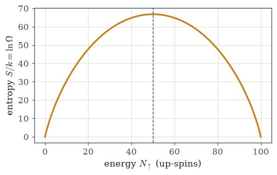
Fig. 415 The entropy \(S/k=\ln\Omega\) of a paramagnet (\(N=100\) spins) against its energy \(N_\uparrow\). It vanishes at the extremes (all down or all up is one microstate) and peaks at half-filling \(N_\uparrow=50\), where \(S_{\max}=\ln\binom{100}{50}\approx66.8\) — the entropy of mixing of §5.3 in physical dress. Below the peak \(S\) rises with energy and the curve is concave; that increasing, concave shape is what forces energy to flow until two magnets in contact reach a common slope — the temperature.

Exercise 4 — Two paramagnets in thermal contact: the sharp peak (worked)

Now the centerpiece. Place two paramagnets \(A\) and \(B\) side by side, able to exchange energy — an up-spin in one can flip down while a down-spin in the other flips up, moving one unit of energy across (Fig. 416). The total energy \(N_\uparrow=N_\uparrow^A+N_\uparrow^B\) is fixed, but it can be partitioned any way. By the postulate every microstate of the combined system is equally likely, so the probability of a given partition \(N_\uparrow^A\) is proportional to the total multiplicity \(\Omega_{\rm total}(N_\uparrow^A)=\Omega_A(N_\uparrow^A)\,\Omega_B (N_\uparrow-N_\uparrow^A)\) Eq. 402 — a product of two large, opposing binomials. The result is a function spectacularly peaked at one partition (Fig. 417), for precisely the \(1/\sqrt N\) reason of §5.3: the product of two multiplicities is as sharp as the binomial was. And the peak sits exactly where energy is shared in proportion to size, \(N_\uparrow^{A\star}=N_\uparrow\,N_A/(N_A+N_B)\).

Part a) For \(N_A=N_B=100\) spins sharing \(N_\uparrow=60\) units of energy, compute \(\ln\Omega_{\rm total}(N_\uparrow^A)\) across every partition in log space — a sum of two ln_omega_paramagnet calls, the one you wrote in Exercise 2 — and locate the peak with numpy.argmax.

Part b) Measure how narrow that peak is: normalize \(\Omega_{\rm total}\) into a probability over partitions and take its standard deviation, reporting the relative width \(\sigma/N_\uparrow^{A\star}\). The figure’s three system sizes show it shrinking as \(1/\sqrt N\).

Part c) Repeat the calculation for unequal magnets, \(N_A=50\) and \(N_B=150\) sharing \(N_\uparrow=80\).

Part d) Confirm both peaks sit at the proportional partition — \(30\) for the equal pair, \(\approx20\) for the unequal one, where the larger magnet takes the larger share.

N_A=100, N_B=100, N↑=60:  peak at N↑^A = 30  (proportional: 30)
peak relative width σ/N↑^A = 0.1083  (∝ 1/√N, the §5.3 sharpness)

N_A=50, N_B=150, N↑=80:  peak at N↑^A = 20  (proportional: 20) — the bigger magnet takes more

Validation 4

✓  energy is shared in proportion to system size at the multiplicity peak   [got 30 vs expected 30 (rtol=1e-06, atol=2)]
✓  the asymmetric paramagnets also share energy in proportion to size   [got 20 vs expected 20 (rtol=1e-06, atol=2)]

True

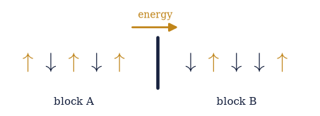
Fig. 416 Two paramagnets in thermal contact. Block \(A\) (\(N_A\) spins) and block \(B\) (\(N_B\) spins) exchange energy: an up-spin flipping down in one is matched by a down-spin flipping up in the other, moving one unit of energy across (amber arrow). Every partition of the fixed total energy is a macrostate; the postulate makes each combined microstate equally likely, so energy flows toward the partition realised by the most microstates.

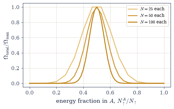
Fig. 417 The total multiplicity \(\Omega_{\rm total}(N_\uparrow^A)/\Omega_{\max}\) of two equal paramagnets (\(N_A=N_B=100\), \(N_\uparrow=60\)), for the full system and for smaller versions. The product of two opposing binomials is razor-sharp at the proportional partition \(N_\uparrow^A=30\), and it narrows as \(1/\sqrt N\) (the §5.3 sharpness): at macroscopic \(N\) essentially every microstate has the energy split in this one ratio. Equilibrium is the overwhelmingly most probable partition, and nothing else is ever seen.

Exercise 5 — The second law from counting (worked)

Here is where a deep idea becomes simple. The second law of thermodynamics says the entropy of an isolated system never decreases. In our picture that is almost a tautology: since \(S_{\rm total}=S_A+S_B=k\ln\Omega_{\rm total}\) Eq. 401, maximizing the total entropy is the same as maximizing the total multiplicity, which is the same as finding the most probable partition. So when we start the two magnets with an unequal split and let energy flow, it flows in the direction that increases \(\Omega_{\rm total}\) — overwhelmingly likely, because that direction has vastly more microstates — until it reaches the peak and stops (Fig. 418). The second law is not an extra postulate; it is the statement that an isolated system drifts to its most probable macrostate, and “irreversibility” is just the fantastically long odds against drifting back.

The simulation below makes the drift visible. Represent the two blocks as one array of \(N_A+N_B\) spins, block \(A\) occupying the first \(N_A\) sites, and let the exchange be a swap: pick two sites at random, and if one is up while the other is down, exchange them. That single move conserves the total energy and carries exactly one unit across whenever the two sites lie in different blocks — the microscopic mechanism of thermal contact, with no knowledge of entropy anywhere in it.

Part a) Confirm that \(S_{\rm total}(N_\uparrow^A)=S_A+S_B\) is maximized at the same partition the multiplicity peaked at in Exercise 4 (numpy.argmax).

Part b) Simulate the approach to equilibrium from a hot-\(A\)/cold-\(B\) start: put all \(60\) units of energy in block \(A\), run \(60{,}000\) random exchanges (numpy.random.default_rng, seeded so the run is reproducible), and record \(N_\uparrow^A\) every \(300\) steps. Write this one yourself — the implementation is the lesson: the second law has to emerge from that blind swapping, and it is the seed of the Metropolis algorithm of §5.10.

Part c) Confirm the trace relaxes to the entropy-maximizing partition and that its late-time fluctuations stay inside the narrow \(1/\sqrt N\) band measured in Exercise 4.

argmax of S_total(N↑^A) = 30  (the equilibrium partition, = the multiplicity peak)

started with all 60 units of energy in A; relaxed to N↑^A ≈ 29 (equilibrium 30)

Validation 5

✓  the total entropy is maximized at the proportional partition — the second law from counting   [got 30 vs expected 30 (rtol=1e-06, atol=1)]
✓  the simulated energy exchange relaxes to the entropy-maximizing partition   [got 28.7667 vs expected 30 (rtol=1e-06, atol=9.74551)]
✓  the late-time fluctuations stay within the narrow 1/√N band about the peak

True

Once Loop Reflect

Fig. 418 The second law, simulated (animated). Starting with all \(60\) units of energy in block \(A\) (\(N_\uparrow^A=60\), far from equilibrium), energy is exchanged one unit at a time by flipping a random up-spin and a random down-spin. The energy in \(A\) (dark) relaxes toward the equilibrium partition \(N_\uparrow^A=30\) (dashed) and then fluctuates about it within the narrow \(1/\sqrt N\) band (amber). Nothing imposes the second law: the spins simply wander, overwhelmingly likely, toward the partition with the most microstates.

Exercise 6 — Temperature emerges (worked)

We have used the word “hotter” loosely; now we earn it. At the equilibrium peak the total entropy is flat, \(dS_{\rm total}/dN_\uparrow^A=0\), which means \(\partial S_A/\partial E_A= \partial S_B/\partial E_B\) Eq. 403. Some quantity, the slope of each magnet’s entropy curve, has become equal — and energy stops flowing precisely when it does. That is what temperature is. We define \(1/T=\partial S/\partial E\), and everything we expect of temperature follows: two bodies in contact reach a common \(\partial S/\partial E\) (they reach a common temperature), and before they do, the body with the smaller slope (the larger \(T\), the hotter one) gives up energy to the body with the larger slope, because that transfer raises the total entropy (Fig. 419). Temperature was never an independent concept; it is the energy-derivative of a count.

With \(E=N_\uparrow\varepsilon\) and \(\varepsilon=1\), that derivative is simply \(\partial S/\partial N_\uparrow\), a numerical gradient of the entropy curve. For two equal blocks the slopes must match at the peak by symmetry alone, which makes that check a weak one; the unequal pair of Exercise 4 (\(N_A=50\), \(N_B=150\), \(N_\uparrow=80\)) carries the real test, since there the two entropy curves are genuinely different functions of energy and have no reason to agree anywhere — except where, by definition, the temperatures are equal.

Part a) Build each block’s entropy curve with the ln_omega_paramagnet you wrote in Exercise 2 and take \(\partial S/\partial E\) of each with numpy.gradient, then plot the two against the shared energy axis of block \(A\).

Part b) Read the two slopes off at the equal pair’s equilibrium partition and confirm they agree.

Part c) Do the same for the unequal pair and confirm that those two genuinely different curves also reach a common \(\partial S/\partial E\) at their equilibrium partition — the equality that is equal temperature.

at equilibrium (N↑^A=30, N↑^B=30):
  ∂S_A/∂E_A = 0.8380
  ∂S_B/∂E_B = 0.8380   (equal → the temperatures match; this defines 1/T)
unequal pair (N_A=50, N_B=150) at its equilibrium (N↑^A=20):
  ∂S_A/∂E_A = 0.3975,  ∂S_B/∂E_B = 0.4027  (still equal)

Validation 6

✓  two genuinely different entropy curves reach equal ∂S/∂E at equilibrium — this defines 1/T   [got 0.397465 vs expected 0.402725 (rtol=1e-06, atol=0.02)]
✓  the equal blocks agree too (by symmetry): ∂S_A/∂E_A = ∂S_B/∂E_B at the peak   [got 0.837995 vs expected 0.837995 (rtol=1e-06, atol=0.003)]

True

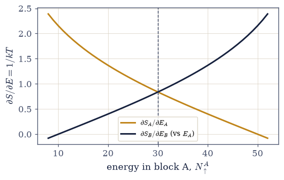
Fig. 419 Temperature as the slope of entropy. The energy-derivative \(\partial S/\partial E=1/kT\) for block \(A\) (amber, falling as \(E_A\) rises) and for block \(B\) (dark, plotted against \(E_B=N_\uparrow-E_A\) so it rises with \(E_A\)) cross at the equilibrium energy \(N_\uparrow^A=30\). Energy flows from the body with the smaller slope (the hotter one) to the body with the larger slope until the slopes — the inverse temperatures — are equal. Temperature is not assumed; it is the energy-derivative of a count.

Exercise 7 — The Boltzmann distribution from a reservoir (worked)

This is the formula the rest of statistical mechanics runs on, and we are going to count it rather than assume it. Take a tiny system — with energy levels \(0,1,2,\dots\) — in contact with a large reservoir, itself a paramagnet holding many units of energy (Fig. 420). The combined system is isolated, so by the postulate every joint microstate is equally likely. The number of joint microstates with the small system at energy \(n\) is just the reservoir’s multiplicity with the rest of the energy, \(\Omega_{\rm res}(Q-n)\), so \(P(n)\propto\Omega_{\rm res}(Q-n)\) Eq. 404. Now the magic: handing \(n\) units to the small system lowers \(\ln\Omega_{\rm res}\) by very nearly a straight line, with slope \(\partial S_{\rm res}/\partial E=1/kT\), so \(\Omega_{\rm res}(Q-n)\propto e^{-n/kT}\). The probability falls off exponentially in energy — the Boltzmann factor — and we obtained it purely by counting the reservoir’s states.

Take the reservoir to be a paramagnet of \(N_R=5000\) spins holding \(Q=1500\) units of energy — below half-filling, so its temperature is an ordinary positive one — and the small system to have the levels \(n=0,1,\dots,25\). For that reservoir the entropy slope has a closed form, \(\beta=\partial S_{\rm res}/\partial E=\ln[(N_R-Q)/Q]\), which is the exponent the counted distribution must reproduce. Nothing below assumes the Boltzmann distribution; it is counted.

Part a) Compute \(P(n)\propto\Omega_{\rm res}(Q-n)\) by direct counting in log space, with the ln_omega_paramagnet you wrote in Exercise 2, and normalize it to a probability.

Part b) Form the Boltzmann prediction \(e^{-\beta n}\) with that closed-form \(\beta\), normalized the same way.

Part c) Confirm the two agree to about a part in \(10^3\) — the master formula of statistical mechanics, obtained by counting a reservoir’s leftover states.

paramagnet reservoir N_R=5000, Q=1500:  β = 1/kT = ln((N_R−Q)/Q) = 0.8473
maximum |P_counted − P_boltzmann| = 4.27e-04

Validation 7

✓  P(E) ∝ e^(−E/kT) falls out of counting the reservoir's microstates — the Boltzmann distribution   [max|Δ| = 0.000427293 (rtol=1e-06, atol=0.002)]

True

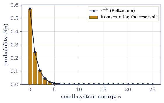
Fig. 420 The Boltzmann distribution, counted not assumed. A small system (energy levels \(0,1,2,\dots\)) in contact with a large paramagnet reservoir; the probability it holds energy \(n\) (amber bars) is proportional to the reservoir’s remaining multiplicity \(\Omega_{\rm res}(Q-n)\), computed by direct counting in log space. It matches the exponential \(e^{-\beta n}\) (dark curve) with \(\beta=1/kT=\ln[(N_R-Q)/Q]\) to about a part in \(10^3\). This Boltzmann factor is the master formula of statistical mechanics, and it is a counting result — the gateway to the canonical ensemble developed later in the volume.

Exercise 8 — Negative temperature and the limits of the picture (student)

Defining temperature as \(1/T=\partial S/\partial E\) has a startling consequence worth meeting, because it sharpens what temperature really is. So far we have worked below half-filling, where the paramagnet behaves normally — adding energy raises the entropy, \(\partial S/\partial E>0\), an ordinary positive temperature. But the paramagnet’s spectrum is bounded: there is a maximum energy, all spins up. Its entropy therefore peaks at half-filling and then falls (Fig. 421). Past the peak — a population-inverted state, more spins up than down — adding energy decreases the entropy, so \(\partial S/\partial E<0\), a formally negative temperature. Far from being colder than absolute zero, such a state is hotter than infinite: it gives up energy to anything with a positive temperature. A system with an unbounded energy spectrum never does this; its entropy rises forever. The lesson is that \(1/T=\partial S/\partial E\), not “average energy,” is the true definition of temperature.

Part a) For a paramagnet of \(N=200\) spins, compute \(S/k=\ln\binom{N}{N_\uparrow}\) across the full energy range with scipy.special.gammaln — writing the three \(\ln\Gamma\) terms out directly this time, so the calculation stands on its own — and take \(\partial S/\partial E\) with numpy.gradient.

Part b) Confirm the slope is positive below half-filling (at \(N_\uparrow=N/4\)) and negative above it (at \(N_\uparrow=3N/4\)): a bounded spectrum admits negative temperature.

paramagnet of N=200 spins:
  ∂S/∂E at quarter energy = +1.0920  (positive: ordinary temperature)
  ∂S/∂E at three-quarter   = -1.0920  (NEGATIVE: hotter than infinite)

Validation 8

✓  a bounded spectrum admits negative temperature — 1/T = ∂S/∂E is the true definition

True

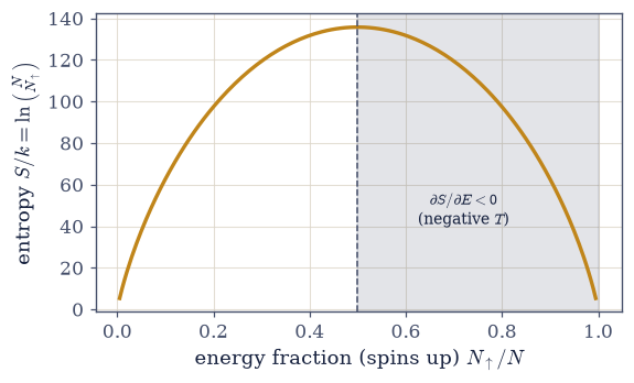
Fig. 421 Entropy of a paramagnet (\(N=200\) spins) against its (bounded) energy. The entropy rises, peaks at half-filling, and falls — because the multiplicity is the binomial \(\binom{N}{N_\uparrow}\), which turns over. On the rising side \(\partial S/\partial E>0\) (ordinary positive temperature); past the peak (shaded), where more spins point up than down, \(\partial S/\partial E<0\), a formally negative temperature that is hotter than infinite. The true definition of temperature is the slope \(1/T=\partial S/\partial E\), not the energy — a distinction a bounded spectrum makes unavoidable.

Exercise 9 — Counting is statistical mechanics

Look back at what one postulate and the counting of three notebooks have built. We assumed only that every accessible microstate of an isolated system is equally likely — the microcanonical ensemble. From the binomial multiplicity of a genuinely classical system, the two-state paramagnet (§5.1), computed in the log space the counts forced on us (§5.3), we read off entropy as \(S=k\ln\Omega\). Bringing two magnets into contact, the \(1/\sqrt N\) sharpness of §5.3 made the equilibrium partition overwhelmingly probable, and the drift toward it is the second law. The slope of entropy that equalizes there is temperature. And counting a reservoir’s leftover states gave the Boltzmann factor \(e^{-E/kT}\), the formula everything downstream is built from. Not one of these was assumed as physics; each was counted. We have arrived at the foundations of thermodynamics — entropy, irreversibility, temperature — and found them to be combinatorics all along.

The closing check is that two quantities introduced separately are one. Exercise 6 defined \(1/T\) as the energy-derivative of entropy; Exercise 7 pulled a \(\beta\) out of a reservoir’s leftover count, \(\ln[(N-Q)/Q]\). For the paramagnet those must be the same number at the same energy, and if they are, the chain from counting to temperature closes.

Part a) For \(N=4000\) spins at \(N_\uparrow=Q=1200\), take the entropy slope \(\partial S/\partial E\) numerically — numpy.gradient on a short window of \(\ln\Omega\) centred on \(Q\), with the ln_omega_paramagnet you wrote in Exercise 2 — and form the Boltzmann exponent \(\ln[(N-Q)/Q]\) alongside it.

Part b) Confirm with np.allclose that they agree: the single \(1/kT\) that ties counting to temperature.

paramagnet N=4000, N↑=1200:
  β from the entropy slope ∂S/∂E = 0.84706
  β from the Boltzmann exponent   = 0.84730
  they agree: True

temperature, entropy, and irreversibility were counting all along

Validation 9

✓  the entropy slope ∂S/∂E and the Boltzmann exponent are one quantity, 1/kT — counting becomes temperature   [got 0.84706 vs expected 0.847298 (rtol=0.001, atol=1e-09)]

True

Notebook summary

From one postulate — the microcanonical ensemble — and the counting of §5.1–§5.3, this notebook built the conceptual core of statistical mechanics, and computed every step exactly with a genuinely classical system, the two-state paramagnet.

• Microstates and the postulate Eq. 398, Eq. 399: every accessible microstate of an isolated system is equally likely (the microcanonical ensemble), so a macrostate’s probability is its multiplicity.

• The paramagnet Eq. 400: \(\Omega(N,N_\uparrow)=\binom{N}{N_\uparrow}\), exactly the binomial / combinations count of §5.1, computed as \(\ln\Omega\) via scipy.special.gammaln because the count overflows (the §5.3 lesson).

• Entropy Eq. 401: \(S=k\ln\Omega\) is extensive (\(\ln\Omega(2N,2N_\uparrow)\to2\ln \Omega(N,N_\uparrow)\)) and maximal at half-filling (\(S_{\max}=\ln\binom{100}{50}\approx66.8\)).

• The second law Eq. 402: \(\Omega_{\rm total}(N_\uparrow^A)=\Omega_A\Omega_B\) is sharply peaked (the \(1/\sqrt N\) sharpness) at proportional energy sharing (\(N_\uparrow^A=30\) for equal magnets, \(20\) for \(50/150\)); energy relaxes there via spin flips, and that drift is the second law.

• Temperature Eq. 403: at the peak \(\partial S_A/\partial E_A=\partial S_B/ \partial E_B\); \(1/T=\partial S/\partial E\) defines temperature.

• The Boltzmann distribution Eq. 404: counting a paramagnet reservoir’s leftover states gives \(P(E)\propto e^{-E/kT}\), with \(\beta=\ln[(N_R-Q)/Q]\) — the master formula, counted not assumed. The bounded paramagnet spectrum even admits negative temperature past half-filling, underscoring that \(1/T=\partial S/\partial E\) is the true definition.

We have arrived at the foundations of thermodynamics by counting. But why is an average over all of phase space the right thing to compute? §5.5 next examines the ergodic hypothesis — that a single trajectory, given time, samples the whole energy surface — which licenses the ensemble method; the canonical ensemble, summing the Boltzmann factor into the partition function, follows later in the volume.

Outlook

• Why the ensembles are valid: ergodicity (§5.5). What we measure is a time average along one trajectory; what an ensemble computes is an average over phase space. The ergodic hypothesis says they agree — demonstrable for a chaotic system, and breakable for an integrable one.

• The canonical ensemble. Summing the Boltzmann factor counted here over a system’s states into the partition function \(Z\) turns \(\ln Z\) into a generating function for energy, entropy, free energy, and heat capacity — the machinery built later in the volume on this notebook’s Boltzmann bridge.

• The other derivatives of entropy (§5.6). Pressure and chemical potential as \(\partial S/\partial V\) and \(\partial S/\partial N\), and the fundamental thermodynamic relation \(dE=T\,dS-P\,dV+\mu \,dN\) — the rest of thermodynamics from the same \(S=k\ln\Omega\).

• Monte Carlo and the Ising model (§5.10). The spin-exchange simulation here is the seed of the Metropolis algorithm and the interacting Ising magnet, whose heat capacity genuinely diverges at a phase transition — the capstone of the volume.

• Quantum statistics (Volume VII). The same counting for indistinguishable particles gives Fermi–Dirac and Bose–Einstein — once Volume VI builds the quantum mechanics behind it.

• Cross-reference §5.1 (the binomial count), §5.3 (log space, entropy, the \(1/\sqrt N\) sharpness).

Take this notebook with you

Use the download button (↓) in the toolbar above to save this notebook and run it yourself. The published notebooks ship without worked solutions; if you would like the reference solutions — to teach from or to check your own work — get in touch: hello@ramador.me.