


3.1 Coulomb’s Law and the Electric Field#
Notebook overview#
Volume III opens by changing the question. Mechanics tracked particles; here the protagonist is the field, a quantity defined at every point of space that a charge placed there would feel. Coulomb’s inverse-square law is the seed, but the moment there is more than one charge the interesting object is no longer a force between two bodies: it is the whole vector field \(\mathbf E(\mathbf r)\) filling space, the superposition of every source. Learning to build, plot, and probe that field numerically is the real subject of this notebook, and the toolbox the rest of the volume leans on.
We will represent a field as arrays on a grid, add fields by superposition, trace field lines by integrating a streamline, and compute the flux of a field through a surface, which turns out to equal the enclosed charge over \(\varepsilon_0\) and previews Gauss’s law (§3.3). Along the way we meet the point charge in its honest mathematical clothing, the Dirac delta, developed not as an assertion but as the limit of a narrowing Gaussian. That idealisation is what makes the Green’s-function solution of Poisson’s equation possible in §3.4, where \(\nabla^2(1/r) = -4\pi\,\delta^3(\mathbf r)\) makes the point charge the fundamental solution. We thread the delta through the volume rather than isolating it.
Everything is in SI units: \(\varepsilon_0 = 8.854\times10^{-12}\,\)F/m and \(k = 1/4\pi\varepsilon_0 \approx 8.99\times10^9\,\)N·m²/C². Electrostatic fields do not move, so every figure here is a faithful static plot: field lines at equal angular spacing (whose density then encodes \(|\mathbf E|\)), or arrows whose length and colour encode \(|\mathbf E|\). A still picture shows a vector field better than motion would.
How to read the checks. Each exercise ends with a
validatecall against an independent fact: an inverse-square ratio, a symmetry cancellation, a flux that matches \(q/\varepsilon_0\), a closed-form field. A ✓ is strong evidence; a ✗ is a prompt to locate the discrepancy, not a verdict.
Theory in brief#
Coulomb’s law and the electric field#
Two point charges \(q_1, q_2\) separated by \(\mathbf r\) (pointing from \(q_1\) to the field point) repel or attract along the line joining them, with a force that falls as the inverse square of the distance:
Dividing out a test charge \(q_{\text{test}}\) removes it from the discussion and leaves a property of space alone, the electric field:
the field of a single point charge \(q\). It is defined everywhere (except at the charge), and a test charge dropped in merely samples it. Numerically we represent \(\mathbf E\) as a pair of component arrays evaluated on a grid.
Superposition#
Maxwell’s equations are linear, so fields add. The field of a collection of charges is the vector sum of their individual point-charge fields, and for a continuous distribution \(\rho(\mathbf r')\) the sum becomes an integral:
Linearity is what makes electrostatics tractable: build the field of anything by adding the fields of its parts.
Field lines#
A field line is a curve everywhere tangent to \(\mathbf E\). Parametrising it by arc length \(s\) gives the unit-speed streamline
which we integrate as an ODE. Field lines begin on positive charges and end on negative ones, and their local density encodes the field strength.
The dipole#
Two opposite charges \(\pm q\) separated by a small displacement \(\mathbf a\) (from \(-q\) to \(+q\)) form a dipole, with dipole moment
The far field falls as \(1/r^3\), one power faster than a single charge, because the charges nearly cancel (Griffiths [Gri17], ch. 3, carries the expansion out in full). The ideal (point) dipole is the limit \(a\to0\) at fixed \(p\); for finite \(a\) the on-axis field carries a small correction we will see explicitly.
The point charge as a delta source#
A point charge is an idealisation: a finite charge \(q\) squeezed to a single point. Its charge density is written with the three-dimensional Dirac delta,
which is not a function but a distribution, defined by its sifting property \(\int f(\mathbf r)\,\delta^3(\mathbf r - \mathbf r_0)\,d^3r = f(\mathbf r_0)\). One realises it as the limit of nascent functions: a Gaussian of unit integral whose width \(w\to0\) so that the peak diverges while the area stays \(1\). The delta is the bridge to the Green’s-function solution of Poisson’s equation in §3.4, where \(\nabla^2(1/r) = -4\pi\,\delta^3(\mathbf r)\) makes the point charge the fundamental solution of electrostatics.
Setup#
Setup holds the data — the SI constants \(\varepsilon_0\) and \(k = 1/4\pi\varepsilon_0\),
the nanocoulomb charge scale, the two conventional charge colours — and a single
instrument, a square grid builder for the field maps. This notebook’s own machinery is
not here: you write the point-charge field E_point in Exercise 1 and the
superposition E_field in Exercise 2, and every later exercise is a question asked of
those two.
The Setup below holds this notebook’s data and instruments — nothing you are asked to build. It is collapsed so the building stays yours; expand it whenever you want the details.
ε₀ = 8.8542e-12 F/m
k = 1/4πε₀ = 8.9876e+09 N·m²/C²
Exercise 1 — The field of a point charge#
The whole volume rests on one field, so we start by building it and confirming it behaves. A single charge produces a purely radial field whose magnitude obeys the inverse-square law of Eq. 187 and Eq. 188, the fingerprint we check first.
Written out in Cartesian components, the field Eq. 188 of a charge \(q\) sitting
at \(\mathbf r_0 = (x_0, y_0)\), evaluated in the \(z = 0\) plane, is
\(k q\,(x - x_0)/d^3\) and \(k q\,(y - y_0)/d^3\) with \(d = |\mathbf r - \mathbf r_0|\).
It diverges at the charge itself, and the honest thing to do numerically is to let
that divergence appear as inf/nan (silence NumPy with numpy.errstate) and leave
the masking to whoever plots it, rather than smoothing the singularity away where it
cannot be seen. The configuration below is a single charge \(q = 1\,\)nC at the origin.
Write
E_point(q, r0, X, Y), returning the two in-plane components of that field in V/m on the coordinate gridsX,Y. Write this one yourself — the implementation is the lesson: this force law is the seed of the whole volume.Sample the magnitude at \(r = 0.1, 0.2, 0.4\,\)m along the \(x\)-axis and verify that halving the distance quadruples the field, i.e. \(E(0.1)/E(0.2) = 4\).
Draw the field over \([-0.5, 0.5]^2\,\)m as lines seeded at equal angles around the charge (Fig. 184), whose density then encodes \(|\mathbf E|\).
|E| at r = 0.1, 0.2, 0.4 m:  [898.75517862 224.68879465  56.17219866] V/m
E(0.1)/E(0.2) = 4.0000   E(0.2)/E(0.4) = 4.0000   (expect 4)
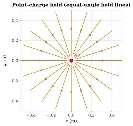
Fig. 184 Field of a point charge \(q=1\,\)nC at the origin, drawn as field lines at equal angular spacing (ecp.draw.radial_field_lines). Equal angle means equal flux per line, so the areal line density falls as \(1/r\) in this plane (and \(1/r^2\) in 3-D), faithfully encoding the inverse-square decay of \(|\mathbf E|\) (Eq. eq-field). A streamplot would place lines by an algorithm whose density carries no such physical meaning.#
Validation 1#
✓ the point-charge field falls as 1/r² [got 4 vs expected 4 (rtol=0.001, atol=1e-09)]
True
Exercise 2 — Superposition and symmetry#
Fields add, and adding them makes symmetry visible. With two identical charges placed symmetrically about the origin, any point on the perpendicular bisector feels two contributions whose sideways parts are mirror images and must cancel, leaving a purely transverse field on the axis. This is superposition Eq. 189 doing the bookkeeping that, by hand, would be a vector diagram.
Because Maxwell’s equations are linear, “the field of many charges” needs no new physics and no new formula: it is the plain sum Eq. 189 of the single-charge fields, term by term on the same grid. That one line of arithmetic is what turns Exercise 1’s force law into a tool for arbitrary sources, so it is worth writing rather than importing. The configuration here is \(q = +1\,\)nC at \((-0.1, 0)\,\)m and \(q = +1\,\)nC at \((+0.1, 0)\,\)m.
Write
E_field(charges, X, Y), which takes a list of(q, (x0, y0))entries and returns the summed in-plane components on the grid, each term evaluated with theE_pointyou wrote in Exercise 1. Write this one yourself — the implementation is the lesson.Confirm that along the \(y\)-axis (the perpendicular bisector) the \(x\)-component vanishes by symmetry.
Map the total field of the pair (Fig. 185).
max |Ex| on the y-axis = 0.00e+00 V/m   (expect 0)
typical |Ey| there      = 2.30e+02 V/m
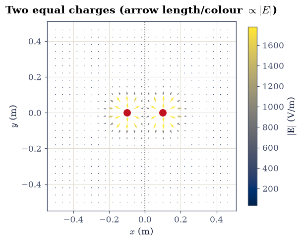
Fig. 185 Field of two equal charges \(q=+1\,\)nC at \((\mp0.1, 0)\,\)m, drawn with ecp.draw.field_quiver: each arrow’s length and colour encode \(|\mathbf E|\) (clipped near the charges), so the picture carries true field strength rather than a streamplot density artefact. On the \(y\)-axis the horizontal components cancel by symmetry, leaving the field along \(y\).#
Validation 2#
✓ the transverse field cancels on the symmetry axis [max|Δ| = 0 (rtol=1e-06, atol=1e-09)]
True
Exercise 3 — The electric dipole#
Bring two opposite charges close together and the monopole fields nearly cancel, leaving a characteristic field that falls as \(1/r^3\) (Eq. 191). The dipole is the first term in the systematic description of any neutral charge distribution (the multipole expansion of §3.5), so its signature is worth meeting directly.
The configuration is \(+1\,\)nC at \((0, +0.01)\,\)m and \(-1\,\)nC at \((0, -0.01)\,\)m: a separation \(a = 0.02\,\)m and a dipole moment \(p = qa\).
Compute the on-axis field at \(z = 0.1, 0.2\,\)m with the
E_fieldyou wrote in Exercise 2.Confirm the far-field \(1/r^3\) falloff (\(E(0.1)/E(0.2) = 8\)).
Compare the magnitude with the ideal-dipole formula \(2kp/r^3\). The small gap is the finite-separation correction: the ideal formula is the \(a\to0\) limit.
on-axis |E| at z = 0.1, 0.2 m:  [366.8014197   45.16329313] V/m
E(0.1)/E(0.2) = 8.122   (expect 8 for 1/r³)
ideal 2kp/r³  at those z:       [359.50207145  44.93775893] V/m
finite-separation excess at z=0.1: 2.0%
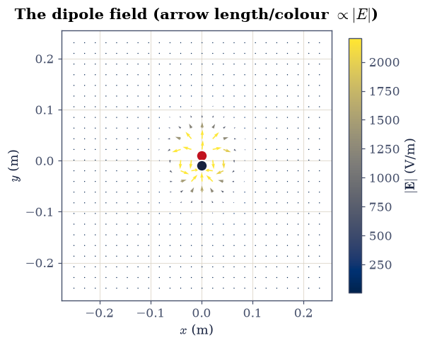
Fig. 186 Field of a dipole (\(+1\,\)nC at \((0,+0.01)\), \(-1\,\)nC at \((0,-0.01)\,\)m), drawn with ecp.draw.field_quiver: arrow length and colour encode \(|\mathbf E|\). The field springs from \(+q\) (red) and returns to \(-q\) (blue), and away from the pair it falls as \(1/r^3\), faster than a single charge.#
Validation 3#
✓ the dipole far-field falls as 1/r³ [got 8.12167 vs expected 8 (rtol=0.05, atol=1e-09)]
True
Exercise 4 — Tracing field lines#
A field map shows direction at sampled points; a field line stitches those directions into a continuous curve, integrating Eq. 190 from a seed point. Seeding the lines at equal angles around the positive charge sends equal flux down each, so the resulting line density is itself a faithful picture of the field strength.
Tracing one costs an ODE solve. Normalising the field to a unit vector makes arc
length the parameter, so the solver takes steps of distance rather than of field
strength and does not crawl where \(|\mathbf E|\) is small. The line has to be told
where to stop, and the natural stopping point is the sink charge: a terminal event
(a function of position that changes sign when the line enters a small capture radius
around \(-q\), with terminal = True and direction = -1) ends each integration
exactly there instead of letting it overshoot into the singularity. The dipole is the
one from Exercise 3.
Write
line_rhs(s, r), the right-hand side \(d\mathbf r/ds = \mathbf E/|\mathbf E|\) of Eq. 190 for that dipole, evaluating \(\mathbf E\) with theE_fieldyou wrote in Exercise 2 and returning zero where the field vanishes. Write this one yourself — the implementation is the lesson.Seed twelve points at equal angles on a small circle around the positive charge and integrate each with
scipy.integrate.solve_ivp(a finemax_step,rtol=1e-8,atol=1e-10,dense_output=True), stopping on the terminal event at \(-q\) and resampling each line uniformly in arc length.Draw the completed lines as a static diagram (Fig. 187): every line that leaves \(+q\) arrives at \(-q\).
field line 0 ends at [ 0.00399978 -0.01004208], distance to −q = 0.0040 m
With the lines traced, draw them as a single static diagram: each curve in full, the charges as fixed markers.
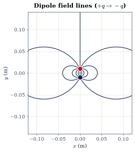
Fig. 187 Static field lines of the dipole, each traced from a seed equally spaced in angle around \(+q\) by integrating \(d\mathbf r/ds=\mathbf E/|\mathbf E|\) (Eq. eq-fieldline) until it reaches \(-q\). Equal-angle seeding carries equal flux down each line, so the line density is physically faithful. Every line leaves \(+q\) (red) and ends on \(-q\) (blue), the defining property of electrostatic field lines.#
Validation 4#
✓ a field line seeded near +q terminates near −q [line end is 0.0040 m from −q]
True
Exercise 5 — The point charge as a delta source#
A point charge holds a finite charge at a single point, so its density Eq. 192 cannot be an ordinary function: it must be zero everywhere yet integrate to \(q\). The Dirac delta captures this as a limit. The Gaussian \(g_w(x) = \exp(-x^2/2w^2)/(w\sqrt{2\pi})\) has unit integral for every width \(w\), and as \(w\to0\) its peak diverges while the area stays exactly \(1\). That limiting object, defined by the sifting property \(\int f(x)\,\delta(x)\,dx = f(0)\), is the delta; in three dimensions \(\rho(\mathbf r) = q\,\delta^3(\mathbf r - \mathbf r_0)\).
The four widths sampled below are \(w = 1, 0.3, 0.1, 0.03\).
Confirm with
numpy.trapezoidthat \(\int g_w\,dx = 1\) at every width while the peak grows as \(1/w\).Plot the four Gaussians superposed on one axes (Fig. 188): the narrowing curves show the diverging peak and the constant unit area at a glance.
w      : [1.   0.3  0.1  0.03]
∫g dx  : [1. 1. 1. 1.]  (expect 1)
peak   : [ 0.399  1.33   3.989 13.298]
peak·w : [0.3989 0.3989 0.3989 0.3989]  (constant 1/√2π = 0.3989)
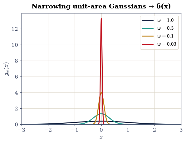
Fig. 188 The nascent delta as four unit-area Gaussians \(g_w(x)=e^{-x^2/2w^2}/(w\sqrt{2\pi})\) for \(w=1,0.3,0.1,0.03\), superposed. As \(w\) shrinks the curve narrows and its peak grows as \(1/w\), yet the area under each stays exactly \(1\): the limit that defines the Dirac delta \(\delta(x)\) (Eq. eq-delta).#
Validation 5#
✓  every nascent-delta Gaussian has unit integral as it narrows   [max|Δ| = 1.97318e-09 (rtol=0.001, atol=1e-09)]
✓  the nascent-delta peak grows as 1/w   [max|Δ| = 5.55112e-17 (rtol=1e-06, atol=1e-09)]
True
Exercise 6 — Gauss’s law previewed: flux of a point charge (student exercise)#
Here is the integral that organises all of electrostatics, and it is yours to compute. The flux of \(\mathbf E\) through a closed surface, \(\oint \mathbf E\cdot d\mathbf A\), measures the field streaming outward through it. For a point charge the inverse-square falloff of the field and the \(r^2\) growth of a sphere’s area cancel exactly, so the flux equals \(q/\varepsilon_0\) regardless of the sphere’s radius. That radius-independence is the integral signature of the delta source and the gateway to Gauss’s law (§3.3).
Doing the surface integral numerically means parametrising the sphere by \((\theta, \varphi)\): the surface point is \(\mathbf r = R(\sin\theta\cos\varphi, \sin\theta\sin\varphi, \cos\theta)\), the full 3-D point-charge field there is \(k q\,\mathbf r/R^3\), the outward unit normal is \(\hat{\mathbf n} = \mathbf r/R\), and the area element is \(dA = R^2\sin\theta\,d\theta\,d\varphi\) — the \(\sin\theta\) is the whole geometry of the sphere and is the term most often dropped. The charge is \(q = 1\,\)nC at the origin, the spheres are concentric with \(R = 0.2, 0.5, 1.0\,\)m.
Write
flux_through_sphere(R, q, n_theta=240, n_phi=480), evaluating \(\oint \mathbf E\cdot d\mathbf A\) with a doublenumpy.trapezoidover that \((\theta, \varphi)\) grid. Write this one yourself — the implementation is the lesson.Confirm the flux equals \(q/\varepsilon_0\) at every radius.
Because the check tests the flux, a ✗ means “re-examine the surface integral or the field,” never a plotting issue.
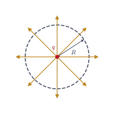
Fig. 189 The Gauss-law setup: a point charge \(q\) (red) at the centre of a spherical Gaussian surface of radius \(R\) (dashed great circle). The field (amber arrows) is radial and crosses the surface normally everywhere, so the flux \(\oint\mathbf E\cdot d\mathbf A\) collects all the field leaving the enclosed charge, equal to \(q/\varepsilon_0\) for any \(R\).#
q/ε₀ = 1.1294e+02 V·m
R = 0.2 m:  flux = 1.1294e+02 V·m,  flux/(q/ε₀) = 0.99999
R = 0.5 m:  flux = 1.1294e+02 V·m,  flux/(q/ε₀) = 0.99999
R = 1.0 m:  flux = 1.1294e+02 V·m,  flux/(q/ε₀) = 0.99999
Validation 6#
✓ the flux through any enclosing sphere is q/ε₀, independent of radius [max|Δ| = 1.43987e-05 (rtol=0.001, atol=1e-09)]
True
Exercise 7 — A continuous distribution: the charged ring#
Real sources are continuous, and superposition Eq. 189 handles them by integration. A uniformly charged ring is the cleanest case: by symmetry its on-axis field is purely axial and has a tidy closed form, \(E_z = kQz/(z^2+R^2)^{3/2}\), against which we can check a numerical integral over the distribution.
The ring makes the azimuthal integral unusually transparent. Every element of the ring lies the same distance \(d = \sqrt{R^2 + z^2}\) from an on-axis field point, and the elements come in diametrically opposite pairs whose radial contributions cancel, so only the axial component survives: with a charge per radian \(\lambda = Q/2\pi\), the integrand \(dE_z/d\varphi = k\lambda z/d^3\) is constant in \(\varphi\). The source is a ring of radius \(R = 0.05\,\)m carrying total charge \(Q = 1\,\)nC in the \(z = 0\) plane.
Write
Ez_ring_numeric(z, n_phi=720), integrating that superposition Eq. 189 over the azimuth withnumpy.trapezoid. Write this one yourself — the implementation is the lesson.Confirm it matches the closed form \(E_z = kQz/(z^2+R^2)^{3/2}\) at \(z = 0.02, 0.05, 0.1, 0.2\,\)m.
Fig. 191 shows the field in a plane through the axis, built by superposing many point charges around the ring.
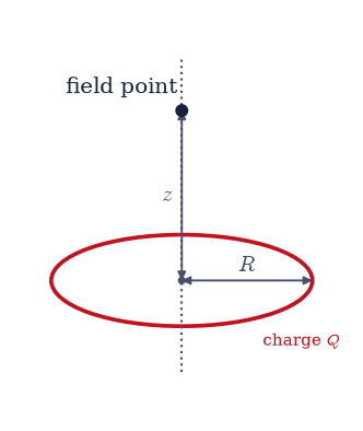
Fig. 190 The charged ring seen obliquely: a circle of radius \(R\) carrying total charge \(Q\), lying in a plane, with its symmetry axis drawn vertically (dotted). The on-axis field point sits a distance \(z\) above the centre; by symmetry the net field there points along the axis. This is the geometry the on-axis integral and Fig. 191 describe.#
z (m)        : [0.02 0.05 0.1  0.2 ]
E_z numeric  : [1150.99756436 1271.03176285  643.09685585  205.15778729]
E_z closed   : [1150.99756436 1271.03176285  643.09685585  205.15778729]
max rel. diff: 4.44e-16
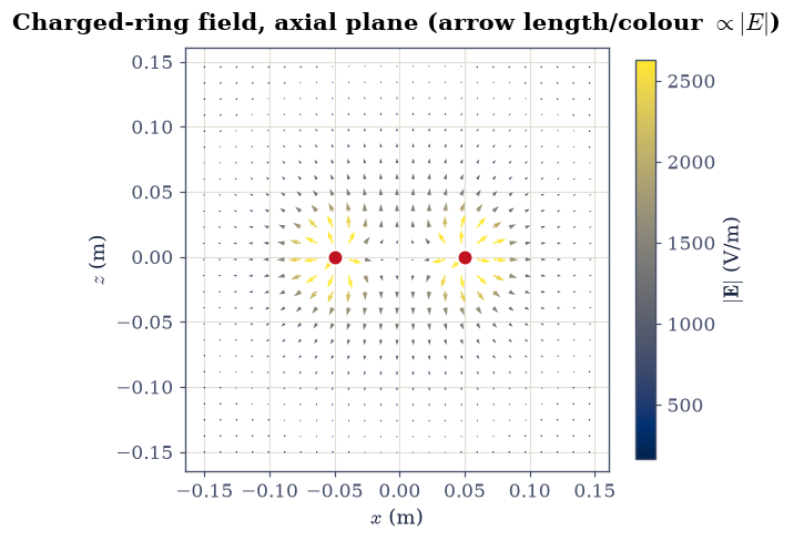
Fig. 191 Field of a uniformly charged ring (radius \(0.05\,\)m, charge \(1\,\)nC) in the plane containing its axis, drawn with ecp.draw.field_quiver (arrow length and colour ∝ \(|\mathbf E|\)). This is a 2-D slice: the red marks at \(x=\pm0.05\,\)m are where the ring pierces the plane, not two point charges. On the axis (\(x=0\)) the field is purely axial, matching the closed form \(E_z=kQz/(z^2+R^2)^{3/2}\) checked above.#
Validation 7#
✓ the numerically integrated ring field matches the closed form [max|Δ| = 2.27374e-13 (rtol=0.0001, atol=1e-09)]
True
Exercise 8 — Numerical divergence of E (synthesis, forward to 3.3)#
One last tool, introduced briefly and developed fully in §3.3. Gauss’s law has a local form, \(\nabla\cdot\mathbf E = \rho/ \varepsilon_0\), which says the field has sources exactly where charge sits and is divergence-free in empty space. We can compute \(\nabla\cdot\mathbf E\) numerically from the field samples with finite differences and watch it vanish away from the charge.
Two grid decisions carry the whole experiment. An even number of points per axis
keeps the origin between samples, so no node sits on the singular charge; and the
verdict is read off an empty-space shell \(0.3 < r < 0.6\,\)m, far enough from the
source that the field is smooth on the grid scale and inside the box, since
numpy.gradient falls back to one-sided, first-order differences on the boundary.
“Zero” for a numerical derivative is relative, so the divergence is compared with
the size of the individual terms \(|\partial_x E_x| + |\partial_y E_y| +
|\partial_z E_z|\) that cancel to produce it.
Evaluate the point-charge field on such a grid and take its numerical divergence with
numpy.gradient.Confirm it is negligible compared with the size of its own derivative terms in that shell.
The spike of divergence at the charge is the delta of Eq. 192, made precise in §3.3.
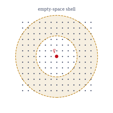
Fig. 192 The divergence-sampling geometry, a 2-D slice of the 3-D grid: the point charge \(q\) (red) sits off every grid node, and \(\nabla\cdot\mathbf E\) is taken by finite differences on the grid. The shaded annulus is the empty-space shell \(0.3<r<0.6\,\)m where \(\nabla\cdot\mathbf E\) should vanish, kept clear of the singular source and of the one-sided box edges.#
empty-space shell 0.3 < r < 0.6 m:
  RMS |∇·E| / RMS(|∂Ex|+|∂Ey|+|∂Ez|) = 3.881e-03
  the divergence is 258× smaller than its own derivative terms there
Validation 8#
✓ the point-charge field is divergence-free in empty space (∇·E ≈ 0 away from the source) [RMS relative divergence in the empty-space shell = 3.881e-03]
True
Notebook summary#
The point-charge field \(\mathbf E=kq\hat{\mathbf r}/r^2\) and its inverse-square fall (\(E(0.1)/E(0.2)=4\)), with superposition cancelling components by symmetry.
The dipole’s on-axis field \(\propto 1/r^3\) (\(E(0.1)/E(0.2)=8\)); field lines traced from \(d\mathbf r/ds=\mathbf E/|\mathbf E|\) and seeded at equal angles, so the line density faithfully encodes \(|\mathbf E|\).
The Dirac delta built as a unit-area Gaussian sequence; the flux of a point charge integrating to \(q/\varepsilon_0\) (a Gauss’s-law preview); the charged ring’s on-axis field; and \(\nabla\cdot\mathbf E\) taken numerically with
numpy.gradient, the local law developed in §3.3.Tools introduced:
ecp.draw.radial_field_linesandecp.draw.field_quiverfor physically faithful field plots, never astreamplotdensity artefact.
Outlook#
More elaborate distributions. The same superposition integral handles surfaces and volumes; solid-angle arguments often replace the integral with a geometric picture.
Earnshaw’s theorem. Because \(\nabla\cdot\mathbf E = 0\) in empty space, no arrangement of fixed charges can trap another charge in stable equilibrium, a clean impossibility result that echoes the saddle-point arguments of §2.7.
Derivatives of the delta. The ideal dipole is \(-\mathbf p\cdot\nabla\delta\), the first in a tower of distributional derivatives that organise the multipole expansion of §3.5.
Forward links. The potential (§3.2) trades this vector field for a scalar; Gauss’s law (§3.3) makes the flux of this notebook a law; and the Green’s-function solution of Poisson’s equation (§3.4) rests on \(\nabla^2(1/r) = -4\pi\,\delta^3(\mathbf r)\), which makes the point charge the fundamental solution of electrostatics.