


0.11 Random Numbers and Monte Carlo Integration#
Notebook overview#
Every stochastic computation in this course, from the statistical mechanics of Volume V to the path-integral Monte Carlo of Volume VII, rests on two ideas this notebook builds from nothing: that a deterministic computer can manufacture numbers which behave random, and that averages over such numbers converge on integrals. Neither is obvious. The first is a small miracle of number theory with famous failures (we will reproduce the most famous one, in three dimensions, where it falls into fifteen flat planes); the second is the law of large numbers wearing its computational face, with an error that shrinks as \(1/\sqrt N\) no matter how many dimensions the integral lives in. That dimension-independence is the whole point: the quadrature rules of §0.3 are unbeatable on a line and hopeless in thirty dimensions, and Monte Carlo is how physics computes where grids cannot go.
We build a linear congruential generator from one line of integer arithmetic and certify it against its designers’ own published test value; break its most notorious cousin; test randomness like a skeptic (moments, bins, correlations); transform uniform deviates into exponential, Gaussian, and semicircular ones; measure the \(1/\sqrt N\) law and set it against the trapezoid rule; estimate hypersphere volumes up to ten dimensions; and end with importance sampling, the doorway through which Volume V’s Metropolis algorithm will walk. The standard references are Numerical Recipes ch. 7 [PTVF07] and Park & Miller’s classic paper [PM88].
A note on reading the checks in this notebook: a validation compares a result to an expected fact. A ✗ does not by itself mean the answer is wrong; it means the output did not match what the check expected, which may be a genuine error, a different-but-valid convention, or a statistical fluctuation pushed past its tolerance. Treat a ✗ as a prompt to locate the discrepancy. Passing is strong evidence, not proof. Statistical checks here use wide (4σ) windows with fixed seeds, so they are deterministic in this notebook as shipped.
Theory in brief#
Pseudorandom numbers. A linear congruential generator (LCG) iterates integer arithmetic,
and returns \(u_k = x_k/m \in [0, 1)\). The sequence is perfectly deterministic (that is what makes results reproducible) and eventually periodic; the art is choosing \(a\), \(c\), \(m\) so the period is long and the numbers pass every statistical test one throws at them. The minimal standard generator of Park & Miller [PM88] uses \(a = 16807\), \(c = 0\), \(m = 2^{31} - 1\) and survives decades of scrutiny; IBM’s RANDU (\(a = 65539\), \(c = 0\), \(m = 2^{31}\)) is the canonical disaster: consecutive triples \((u_k, u_{k+1}, u_{k+2})\) obey the exact integer identity
so every triple lies on one of just fifteen parallel planes in the unit
cube [Mar68]. Modern generators (NumPy’s default PCG64,
reached through numpy.random.default_rng) have periods near \(2^{128}\)
and no such structure; the course’s standing rule of seeding every
generator is precisely the determinism of Eq. 66 used for us.
Transforming distributions. With uniform \(U\) in hand, other densities follow. The inverse transform: if \(F\) is a cumulative distribution function, \(X = F^{-1}(U)\) has density \(F'\); for the exponential distribution \(p(x) = \lambda e^{-\lambda x}\) this reads
The Box–Muller transform manufactures exact Gaussians from two uniforms,
both \(\sim\mathcal N(0,1)\) and independent. And rejection sampling draws from any bounded density \(p\) on \([a, b]\) with no inverse at all: propose \((x, y)\) uniformly in the enclosing rectangle, keep \(x\) when \(y < p(x)\).
Monte Carlo integration. The mean-value estimator turns an integral into an average,
with standard error \((b-a)\,\sigma_f/\sqrt N\), where \(\sigma_f^2\) is the variance of \(f\) under the sampling density. The \(1/\sqrt N\) is the central limit theorem (Volume V derives it as physics in §5.3); its power is what it lacks: any reference to dimension. A product trapezoid grid at \(n\) points per axis costs \(n^d\) evaluations for error \(\mathcal O(n^{-2})\), i.e. error \(\mathcal O(N^{-2/d})\) at total cost \(N\); Monte Carlo’s \(N^{-1/2}\) wins for every \(d > 4\), and in the \(10^{23}\)-dimensional integrals of statistical mechanics it is the only method there is.
Importance sampling. Sampling from a density \(w\) shaped like the integrand slashes the variance:
exact for any \(w > 0\) where \(f \neq 0\), and dramatically better when \(f/w\) is nearly constant. Its limit defines the frontier this notebook stops at: when the ideal weight is a density one cannot sample directly (a Boltzmann factor with an unknown normalization), a cleverer machine is needed. That machine is the Metropolis algorithm, and Volume V builds it where its physics lives (§5.8).
Setup#
Setup holds data and nothing else here: the master seeded generator for the
opening dartboard, and the published parameters of the two historical
generators (Park & Miller’s minimal standard, IBM’s RANDU). This notebook’s
own machinery is not here — you write the linear congruential generator
lcg_sequence in Exercise 2 and the mean-value estimator mc_mean_value
in Exercise 5, the two pieces of code the rest of the notebook runs on. All
randomness is seeded (numpy.random.default_rng with named seeds per
study), so every number and every histogram in this notebook reproduces
exactly. The LCGs are implemented in exact integer arithmetic; floats
appear only when a state is divided by the modulus.
The Setup below holds this notebook’s data and instruments — nothing you are asked to build. It is collapsed so the building stays yours; expand it whenever you want the details.
Exercise 1 — π from darts#
The oldest Monte Carlo computation makes the estimator Eq. 70 visible before any formalism. Throw \(N\) points uniformly into the unit square \([0,1]^2\); the fraction landing inside the quarter disk \(x^2 + y^2 \le 1\) estimates its area \(\pi/4\), because a uniform point’s probability of landing in a region is that region’s area. The count of hits is binomial, so the estimator \(\hat p\) carries the standard error \(\sqrt{\hat p(1-\hat p)/N}\), and \(4\hat p\) estimates \(\pi\) with four times that. Fig. 58 shows the geometry with the first 400 throws.
Part a) With rng.uniform(0.0, 1.0, size=(N, 2)) and \(N = 10^6\), count
hits via the boolean mean of \(x^2 + y^2 \le 1\) (numpy.mean on the
comparison), form \(\hat\pi = 4\hat p\) and its standard error
\(4\sqrt{\hat p(1-\hat p)/N}\), and verify \(|\hat\pi - \pi|\) lies within
\(4\) standard errors (a deterministic check at this seed; the window says
what any seed should satisfy 99.99% of the time).
Part b) Verify the scaling claim coarsely before Exercise 5 measures it properly: with the same binomial formula \(4\sqrt{\hat p(1-\hat p)/N}\) at both sizes, the standard error at \(N = 10^6\), about \(1.6\times10^{-3}\), is ten times smaller than at \(N = 10^4\): 100× the work for 10× the precision. That exchange rate is the price of the method, and Exercise 5’s fitted slope makes it exact.
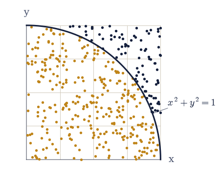
Fig. 58 The dartboard estimator for \(\pi\): 400 points drawn uniformly in the unit square \([0,1]^2\), amber where they land inside the quarter disk \(x^2+y^2\le1\) (of area \(\pi/4\)) and ink where they miss. The hit fraction estimates the area, so four times the fraction estimates \(\pi\), with binomial standard error \(4\sqrt{\hat p(1-\hat p)/N}\).#
pi estimate : 3.141196 ± 0.001642 (pi = 3.141593)
pull : -0.24 sigma
sem at 1e4 : 1.64e-02; at 1e6: 1.64e-03
✓ a million darts estimate π within four binomial standard errors [π̂ = 3.141196 ± 0.001642, pull -0.24σ]
✓ the exchange rate: 100× the samples buy 10× the precision (the 1/√N law, measured coarsely) [got 10.0135 vs expected 10 (rtol=0.05, atol=1e-09)]
True
Exercise 2 — A generator from one multiplication, and a famous corpse#
Where do the “uniform” numbers come from? Equation Eq. 66 is the whole machine, and this exercise builds it and drives three instances of it in exact integer arithmetic: one good, one small enough to see all the way through, one notorious. The claim that a deterministic sequence can behave random is audited in Exercise 3; here we certify the machinery itself, the way its designers did. Their certification is unusually sharp: Park & Miller published the ten-thousandth state of their generator from seed \(x_0 = 1\) precisely so that an implementation could be checked bit-for-bit [PM88], and a period claim can be checked the same way on a generator small enough to exhaust — the Hull–Dobell theorem says an LCG with \(c\) odd and \(a - 1\) divisible by \(4\) visits every residue mod \(m\) exactly once, so \(a = 5\), \(c = 1\), \(m = 32\) must have period exactly \(32\).
Part a) Write lcg_sequence(a, c, m, seed, n), which iterates
Eq. 66 from the state \(x_0 =\) seed and returns the next \(n\)
states \(x_1, \dots, x_n\) as a numpy.int64 array. Keep the loop in exact
Python integer arithmetic ((a * x + c) % m on Python ints neither
overflows nor rounds); every modulus used here is at most \(2^{31}\), so the
states fit int64 with room to spare. Write this one yourself — the
implementation is the lesson: these five lines are the entire source of
randomness for the rest of the exercise.
Part b) Drive it as the Park–Miller minimal standard (\(a = 16807\), \(c = 0\), \(m = 2^{31} - 1\)) from seed \(x_0 = 1\). Verify the first three states are exactly \(16807\), \(282475249\), \(1622650073\), and the ten-thousandth state is exactly \(1043618065\): the certification value Park & Miller published for this purpose [PM88]. Integer arithmetic either reproduces it bit-for-bit or the implementation is wrong; there is no tolerance.
Part c) Periods are finite. For the toy generator \(a = 5\), \(c = 1\),
\(m = 32\) from seed \(7\), generate 64 states and locate
the period as the first index where the state returns to its first value
(numpy.flatnonzero on the equality), verifying it is exactly \(32\), the
maximum possible, and that the first 32 states are 32 distinct residues.
The minimal standard’s period is \(m - 1 = 2^{31} - 2
\approx 2\times10^9\); PCG64’s is \(2^{128}\). A simulation that consumes
more numbers than the period is recycling its own noise.
Part d) The corpse. Drive RANDU (\(a = 65539\), \(c = 0\), \(m = 2^{31}\)) from seed \(1\) and verify the exact integer identity Eq. 67: \((x_{k+2} - 6x_{k+1} + 9x_k) \bmod 2^{31} = 0\) for every \(k\) over \(10^4\) consecutive states. This is why RANDU’s triples fall on fifteen planes: the identity confines them [Mar68]. Then see it: plot 4000 consecutive triples \((u_k, u_{k+1}, u_{k+2})\) viewed edge-on (matplotlib’s 3-D axes at azimuth \(-115°\), elevation \(12°\), where the planes align), beside the same picture for PCG64 triples, and animate a slow rotation of the RANDU cloud: from almost every angle it looks like noise, and from the right one it is fifteen sheets of paper.
PM first three : [16807, 282475249, 1622650073]
PM state 10000 : 1043618065
toy period : 32 (32 distinct residues)
RANDU identity : max residual 0 (exact zero)
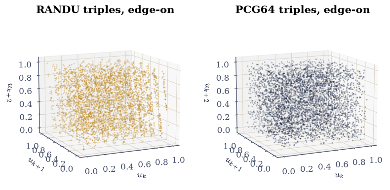
Fig. 59 Consecutive triples \((u_k,u_{k+1},u_{k+2})\) of 4000 RANDU deviates (left) and 4000 PCG64 deviates (right), both viewed from azimuth \(-115°\), elevation \(12°\). From this angle RANDU’s exact recurrence \(x_{k+2}=6x_{k+1}-9x_k \bmod 2^{31}\) confines every triple to one of fifteen parallel planes; the modern generator shows no structure from any angle.#
Fig. 60 Animation of the 4000 RANDU triples of the previous figure under a slow rotation of the viewpoint (elevation fixed at \(12°\), azimuth sweeping \(180°\)): the cloud reads as featureless noise from most angles and collapses into Marsaglia’s fifteen parallel planes as the view aligns with them. The structure is exact, not statistical: every triple obeys the integer recurrence.#
✓ the minimal standard's first three states, exact to the integer [max|Δ| = 0 (rtol=0, atol=0)]
✓ Park & Miller's own certification: state 10,000 from seed 1 is 1043618065, bit-for-bit [got 1043618065]
✓ the Hull–Dobell toy generator achieves its full period, visiting every residue mod 32 exactly once [period 32, distinct 32]
✓ RANDU's fifteen planes are an exact theorem: x_{k+2} = 6x_{k+1} − 9x_k (mod 2³¹) with zero residual over 10⁴ states [max residual 0]
True
Exercise 3 — Testing randomness like a skeptic#
“Behaves random” is a statistical claim, and statistical claims are tested. For genuinely uniform deviates on \([0, 1)\) the moments are \(\langle u^k\rangle = 1/(k+1)\); a histogram of \(B\) equal bins should carry counts whose \(\chi^2 = \sum_b (n_b - N/B)^2/(N/B)\) follows the \(\chi^2\)-distribution with \(B - 1\) degrees of freedom; and consecutive pairs should be uncorrelated, \(\langle u_k u_{k+1}\rangle - 1/4 \to 0\) with standard error of order \(1/\sqrt N\)… each test probes a different way a generator can fail while passing the others (RANDU passes all three and dies only in three dimensions, which is the lesson: tests rule out, never certify).
Part a) Draw \(N = 10^6\) PCG64 deviates (numpy.random.default_rng(23))
and verify the first four moments \(\langle u^k\rangle\), \(k = 1,\dots,4\),
each within \(4\sigma_k/\sqrt N\) of \(1/(k+1)\), where \(\sigma_k^2 =
1/(2k+1) - 1/(k+1)^2\) is the exact variance of \(u^k\).
Part b) Bin the same sample into \(B = 50\) equal bins with
numpy.histogram and verify \(\chi^2\) lies inside the central 99.8% window
of \(\chi^2_{49}\), \([\,\)scipy.stats.chi2.ppf(0.001, 49),
scipy.stats.chi2.ppf(0.999, 49)\(\,]\). Verify the lag-1 correlation
\(\langle u_k u_{k+1}\rangle - 1/4\) is within \(4\cdot(1/4)/\sqrt N\) of zero
(the pair variance for uniforms is \(\mathrm{Var}(u_ku_{k+1}) = 1/9 - 1/16
= 7/144 \approx (0.22)^2\); the \(1/4\) window is comfortably wider).
Part c) Feed the same \(\chi^2\) test (the numpy.histogram binning and
\(\chi^2\) sum of Part b, unchanged) \(10^6\) deviates from the toy
32-period generator of Exercise 2 — the lcg_sequence you wrote there,
run with \(a = 5\), \(c = 1\), \(m = 32\) from seed \(7\), divided by \(32\) (its
\(10^6\) samples are the same 32
values recycled 31,250 times). Verify its \(\chi^2\) exceeds the PCG64 value
by a factor above \(100\): a generator that fails, fails loudly, when the
test matches the failure.
moment pulls (sigma): ['-0.56', '-0.35', '-0.23', '-0.15']
chi2 PCG64 : 49.0 (window [24.0, 85.4])
lag-1 corr : -1.43e-04
chi2 toy : 5.625e+05 (11482x PCG64)
✓ the first four moments of 10⁶ PCG64 deviates sit within 4σ of 1/(k+1), each against its exact variance [pulls ['-0.56', '-0.35', '-0.23', '-0.15']]
✓ the 50-bin χ² lands inside the central 99.8% window of χ²₄₉: flat, but not suspiciously flat [χ² = 49.0 in [24.0, 85.4]]
✓ consecutive deviates are uncorrelated at the 1/√N level [⟨u_k u_(k+1)⟩ − 1/4 = -1.43e-04]
✓ the 32-period toy generator fails the same χ² test by more than two orders of magnitude: recycling is visible [ratio 11482×]
True
Exercise 4 — Manufacturing distributions#
Physics rarely wants uniform numbers; it wants Boltzmann factors, decay times, Gaussian noise. This exercise builds the three standard transformations of the theory section, each validated against facts the construction did not assume.
Part a) Inverse transform, Eq. 68: from \(N = 10^5\) uniform
deviates (numpy.random.default_rng(31)), form \(X = -\ln(1 - U)\)
(exponential, \(\lambda = 1\): the distribution of radioactive decay times
with unit mean life). Verify the sample against the exponential
distribution with the Kolmogorov–Smirnov test,
scipy.stats.kstest(x, "expon"), demanding \(p > 0.01\), and verify the
sample mean sits within \(4/\sqrt N\) of \(1\) (mean and standard deviation of
the unit exponential are both \(1\)).
Part b) Box–Muller, Eq. 69: from two arrays of \(5\times
10^4\) uniforms, build both Gaussian channels \(Z_1, Z_2\), concatenate, and
verify with scipy.stats.kstest(z, "norm") at \(p > 0.01\); verify the
sample variance within \(4\sqrt{2/N}\) of \(1\) (the variance of a sample
variance of \(N\) Gaussians is \(2/N\)).
Part c) Rejection sampling for a density with no closed-form inverse: the Wigner semicircle \(p(x) = \tfrac{2}{\pi}\sqrt{1 - x^2}\) on \([-1, 1]\) (the eigenvalue density of the random matrices of §0.5, one volume early). Propose \((x, y)\) uniformly in \([-1, 1]\times[0, 2/\pi]\), accept when \(y < p(x)\), and verify (i) the acceptance rate equals the area ratio \(\frac{\pi/2\cdot(2/\pi)^2} {2\cdot 2/\pi} = \pi/4\) within \(4\) binomial standard errors, and (ii) the accepted sample’s variance meets the analytic \(\int x^2 p\,dx = 1/4\) within \(4\sigma\) of the sample-variance error. Fig. 61 shows all three histograms on their target densities.
KS p (expon): 0.038; mean 0.9996
KS p (norm) : 0.761; var 1.0001
acceptance : 0.7847 (pi/4 = 0.7854); var 0.2506
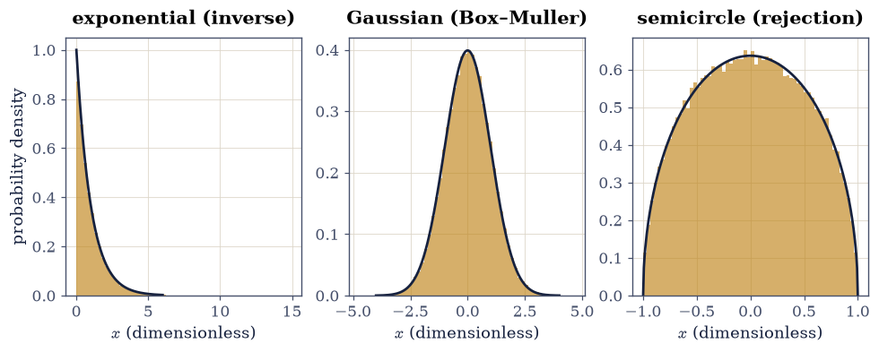
Fig. 61 Three manufactured distributions, each histogram (amber, density-normalized) on its exact target density (ink): the unit exponential \(e^{-x}\) from the inverse transform \(X=-\ln(1-U)\); the standard Gaussian from the Box–Muller transform; and the Wigner semicircle \(\tfrac{2}{\pi}\sqrt{1-x^2}\) from rejection sampling under a uniform envelope. All three consume nothing but uniform deviates.#
✓ the inverse transform delivers the unit exponential: KS accepts and the mean is 1 within 4σ [p = 0.038, mean = 0.9996]
✓ Box–Muller delivers exact standard Gaussians: KS accepts and the variance is 1 within 4σ [p = 0.761, var = 1.0001]
✓ the rejection acceptance rate equals the area ratio π/4 [got 0.784725 vs expected 0.785398 (rtol=0, atol=0.00367621)]
✓ the semicircle sample's variance meets the analytic ∫x²p dx = 1/4 [got 0.250639 vs expected 0.25 (rtol=0.02, atol=1e-09)]
True
Exercise 5 — The 1/√N law, measured#
Now the estimator itself. We integrate a completely explicit target, \(\int_0^1 e^x\,dx = e - 1\), with the mean-value estimator Eq. 70, and measure how its error falls with \(N\): the claim is a power law \(N^{-1/2}\), so on log–log axes the RMS error over repeated runs is a line of slope \(-1/2\). Against it we run the trapezoid rule of §0.3 on the same integral, whose error falls as \(N^{-2}\): in one dimension quadrature wins without contest, and Exercise 6 shows why that verdict reverses in ten.
Part a) Write mc_mean_value(f, a, b, n, generator), returning the
pair (estimate, standard_error): draw \(n\) points uniformly on \([a, b]\)
from the supplied seeded generator, average \(f\) over them, and scale by
\((b - a)\) per Eq. 70; the error bar is
\((b-a)\,\mathrm{std}(f)/\sqrt n\) with the sample standard deviation taken
from the very same draw (numpy.std with ddof=1). Write this one
yourself — the implementation is the lesson: two lines, and every
stochastic method later in this course is a refinement of them.
Part b) At \(N = 10^4\) (numpy.random.default_rng(47)), verify the
estimate lies within \(4\) of its own reported standard errors of
\(e - 1\): the estimator carries its uncertainty with it, and the
uncertainty is honest.
Part c) For \(N \in \{10^2, 10^3, 10^4, 10^5, 10^6\}\), run \(24\)
independent repeats each (seeds \(100\cdot j + i\) so every run is distinct
and reproducible), form the RMS error against the exact \(e - 1\), and fit
\(\log_{10}(\mathrm{RMS})\) vs \(\log_{10} N\) with numpy.polyfit (degree 1,
the fitting machinery of §0.8). Verify the
slope is \(-1/2\) within \(\pm 0.08\).
Part d) Evaluate the trapezoid rule (numpy.trapezoid on a uniform
grid) at the same five \(N\) and fit its slope: \(-2\) within \(\pm 0.1\).
Fig. 62 overlays both laws; the crossing favors the
grid everywhere in one dimension. Keep the figure in mind: Exercise 6
moves the same contest to \(d\) dimensions, where the grid’s exponent decays
as \(-2/d\) and Monte Carlo’s does not move.
single estimate : 1.72995 ± 0.00490 (pull +2.38σ)
MC slope : -0.5221 (expect -0.5)
trapezoid slope : -2.0017 (expect -2)
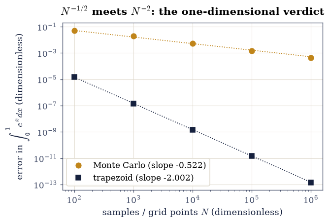
Fig. 62 Convergence of two ways to compute \(\int_0^1 e^x dx=e-1\): the RMS error of the mean-value Monte Carlo estimator over 24 seeded repeats (amber points) falls on the fitted \(N^{-1/2}\) law, while the trapezoid rule on a uniform \(N\)-point grid (ink points) falls on \(N^{-2}\). In one dimension the grid wins without contest; the exponents, not the prefactors, are the story, and only the grid’s exponent degrades with dimension.#
✓ the estimator's own error bar is honest: the estimate sits within 4 of its reported standard errors of e − 1 [pull +2.38σ]
✓ the Monte Carlo error falls as N^(-1/2): the fitted log-log slope over five decades [got -0.522069 vs expected -0.5 (rtol=0, atol=0.08)]
✓ the trapezoid error falls as N^(-2) on the same integral: the one-dimensional benchmark to beat [got -2.00168 vs expected -2 (rtol=0, atol=0.1)]
True
Exercise 6 — Where grids die: volumes in ten dimensions#
The \(d\)-dimensional unit ball has exact volume
a formula with a strange story to tell: against the enclosing hypercube \([-1,1]^d\) of volume \(2^d\), the ball’s share \(V_d/2^d\) collapses with dimension (from \(\pi/4 \approx 0.785\) at \(d = 2\) to \(2.5\times10^{-3}\) at \(d = 10\)): high-dimensional volume concentrates in corners. A product trapezoid grid with even \(10\) points per axis would need \(10^{10}\) evaluations at \(d = 10\); the dart estimator of Exercise 1, generalized verbatim, needs only enough darts for the target precision, because its \(1/\sqrt N\) error never asks what \(d\) is.
Part a) For \(d \in \{2, 4, 6, 8, 10\}\), throw \(N = 4\times10^5\) points
uniformly in \([-1, 1]^d\) (numpy.random.default_rng(50 + d), shape
\((N, d)\)), count the fraction \(\hat p\) with \(\sum_i x_i^2 \le 1\)
(numpy.mean on the row-wise comparison of numpy.sum(x**2, axis=1)),
and estimate \(V_d = 2^d\,\hat p\) with standard error
\(2^d\sqrt{\hat p(1-\hat p)/N}\).
Part b) Verify every estimate against Eq. 72 (via
scipy.special.gamma) within \(4\) standard errors, and verify the
collapse: \(\hat p(d)\) decreases monotonically and \(\hat p(10) < 3\times
10^{-3}\). Fig. 63 shows the estimates riding the
exact curve.
d : [2, 4, 6, 8, 10]
V̂ : ['3.1415', '4.9208', '5.1342', '4.1069', '2.4448']
V : ['3.1416', '4.9348', '5.1677', '4.0587', '2.5502']
pulls: ['-0.04', '-1.20', '-1.22', '+0.95', '-1.33']
hit fraction at d=10: 0.00239
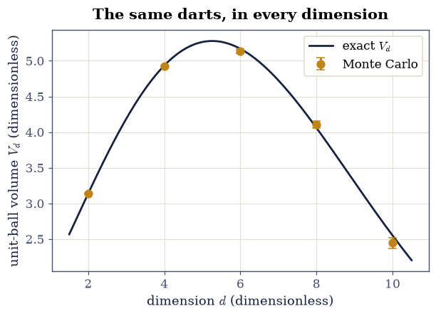
Fig. 63 Monte Carlo estimates of the unit-ball volume \(V_d\) (amber points, \(4\times10^5\) darts per dimension, error bars \(2^d\sqrt{\hat p(1-\hat p)/N}\)) on the exact \(V_d=\pi^{d/2}/\Gamma(d/2+1)\) (ink curve), for \(d=2\) to \(10\). The volume peaks near \(d=5\) and then decays; the estimator’s relative cost is set only by the hit fraction, never by a grid, which is why the same twenty lines of code work at every \(d\).#
✓ all five unit-ball volumes, d = 2 through 10, land within 4σ of π^(d/2)/Γ(d/2+1) [pulls ['-0.04', '-1.20', '-1.22', '+0.95', '-1.33']]
✓ the corner collapse: the ball's share of the hypercube falls monotonically, to 0.25% by d = 10 [p̂(10) = 2.39e-03]
True
Exercise 7 — Importance sampling, and the doorway to Metropolis#
The mean-value estimator wastes samples wherever the integrand is small. Equation Eq. 71 fixes that by sampling where the integrand lives. Our target is the completely explicit
an integrand that is exponentially negligible beyond \(x \approx 10\) yet formally infinite in extent.
Part a) The naive route: truncate at \(L = 25\) (where the integrand is
below \(10^{-8}\)) and apply the mc_mean_value you wrote in Exercise 5 on
\([0, L]\) with
\(N = 10^5\) uniform samples (numpy.random.default_rng(61)). It works, and
wastefully: most samples land where \(e^{-x}\) has already killed the
integrand. Record the estimate and its standard error.
Part b) The importance route, with a weight shaped like the integrand: the Gamma\((2,1)\) density \(w(x) = x\,e^{-x}\), which one samples with the tools already built, as the sum of two independent unit exponentials, \(X = -\ln(1-U_1) - \ln(1-U_2)\) (the inverse transform of Exercise 4, twice; seed \(62\), same \(N\)). The estimator averages \(f(X)/w(X) = \sqrt X\), whose variance under \(w\) is \(\mathbb E[X] - I^2 = 2 - \Gamma(5/2)^2 \approx 0.233\), against the naive route’s \(\approx 7.6\) (after the \(L^2\) factor). Verify both estimates agree with \(\Gamma(5/2)\) within \(4\) of their own standard errors, and verify the variance reduction: the naive standard error exceeds the matched-weight one by a factor above \(5\). The weight did not change the answer (it cannot: Eq. 71 is an identity); it changed the cost of the answer. A first, tempting choice of weight, plain \(w = e^{-x}\), buys almost nothing here (a factor \(1.3\): its ratio \(f/w = x^{3/2}\) is unbounded, so its variance stays large) — this notebook’s own drafting made exactly that mistake, and the variance formula caught it. Matching the weight to the integrand’s shape, not merely its tail, is the craft.
Part c) Push the logic to its end: the perfect weight is the
normalized integrand itself, \(w^\star(x) = x^{3/2}e^{-x}/\Gamma(5/2)\) (the
Gamma\((5/2, 1)\) density, drawn with numpy.random.Generator.gamma(2.5),
seed \(63\)). Then \(f/w^\star = \Gamma(5/2)\) is constant: every sample
returns the exact answer and the estimator’s spread collapses to rounding
(verify the sample standard deviation of the ratios is below \(10^{-12}\)).
The catch is the point: building \(w^\star\) required already knowing the
normalization \(\Gamma(5/2)\), which is the integral. Benchmark everything
against deterministic quadrature, scipy.integrate.quad of
\(x^{3/2}e^{-x}\) on \((0, \infty)\), which agrees with \(\Gamma(5/2)\) to
thirteen digits: in one dimension, quadrature still reigns. The
limitation to carry forward is Part c)’s circle: importance sampling
required a weight we could sample directly. The Boltzmann weight
\(e^{-\beta E(\mathbf s)}/Z\) of statistical mechanics is exactly the weight
one wants and exactly the one no inverse transform reaches (\(Z\) itself is
the unknown). The machine that samples it anyway, one accepted move at a
time, is the Metropolis algorithm, built in
§5.8 where its
physics lives, and refined ever after (checkerboard sweeps in
§5.10,
staging for ring polymers in
§7.21).
This notebook ends at that doorway on purpose.
naive : 1.32654 ± 0.00871
importance : 1.32958 ± 0.00152
perfect w* : ratio spread 2.31e-16 (zero variance)
quad : 1.3293403881762 (Γ(5/2) = 1.3293403881791)
variance-reduction factor: 5.7x
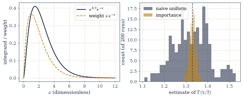
Fig. 64 Importance sampling for \(I=\int_0^\infty x^{3/2}e^{-x}dx=\Gamma(5/2)\): the integrand (ink) against the shape-matched sampling weight \(w(x)=x\,e^{-x}\) (amber, dashed) on the left; on the right, the distribution of 200 independent estimates from \(10^3\) samples each, naive-uniform on \([0,25]\) (ink) versus importance-sampled (amber). Both centre on \(\Gamma(5/2)\) (dashed line); the importance estimator’s spread is several times narrower at identical cost.#
✓ both estimators agree with Γ(5/2) within 4 of their own standard errors: the weight changes cost, never the answer [naive pull -0.32σ, importance pull +0.16σ]
✓ the shape-matched Gamma(2,1) weight cuts the standard error more than 5× at identical N [factor 5.7×]
✓ the perfect weight w* ∝ f has ZERO variance: every sample returns Γ(5/2) exactly — and building it required knowing the answer [ratio spread 2.3e-16]
✓ scipy.integrate.quad confirms Γ(5/2) to thirteen digits: in one dimension, deterministic quadrature still reigns [got 1.32934 vs expected 1.32934 (rtol=1e-12, atol=1e-09)]
True
Notebook summary#
A million uniform darts estimated \(\pi\) within four binomial standard errors, and quadrupling precision cost a hundredfold work: the \(1/\sqrt N\) exchange rate, met before its formalism.
The Park–Miller minimal standard Eq. 66, in exact integer arithmetic, reproduced its designers’ certification bit-for-bit (states \(16807, 282475249, 1622650073\); state \(10{,}000 = 1043618065\)); the Hull–Dobell toy generator achieved its full period of 32; and RANDU’s fifteen planes were verified as the exact theorem Eq. 67, with zero integer residual over \(10^4\) states, then seen edge-on and in rotation.
Randomness testing ruled like a skeptic: four moments within \(4\sigma\), the 50-bin \(\chi^2\) inside the central 99.8% window of \(\chi^2_{49}\), lag-1 correlation at the \(1/\sqrt N\) level, and the 32-period generator failing the same \(\chi^2\) by more than two orders of magnitude.
Uniform deviates became exponential (Eq. 68, KS-accepted, mean \(1\)), Gaussian (Eq. 69, KS-accepted, variance \(1\)), and semicircular (rejection; acceptance rate \(\pi/4\), variance \(1/4\)).
The mean-value estimator Eq. 70 carried an honest error bar and a measured slope of \(-1/2\) over five decades of \(N\), against the trapezoid rule’s \(-2\): the one-dimensional verdict, reversed in high dimension by the unit-ball volumes of Eq. 72, all five within \(4\sigma\) up to \(d = 10\) where the grid could not have been afforded.
Importance sampling Eq. 71 with the shape-matched Gamma\((2,1)\) weight cut the standard error of \(\Gamma(5/2)\) more than fivefold at identical cost (a merely tail-matched \(e^{-x}\) bought a factor \(1.3\): shape is the craft); the perfect weight collapsed the variance to rounding at the price of already knowing the answer; and that circle named the machine this notebook deliberately stops before: Metropolis, built in §5.8.
Outlook#
The central limit theorem as physics. The \(1/\sqrt N\) measured here is derived in §5.3 and becomes the reason thermodynamic quantities are sharp; §5.2 supplies the probability language this notebook used informally.
Markov-chain Monte Carlo. When the weight cannot be sampled directly, Metropolis (§5.8) samples it through a chain of accepted moves, at the price of correlated samples; the autocorrelation bookkeeping that prices that correlation honestly is built in §7.21.
Quasi-random sequences. Low-discrepancy (Sobol) points beat \(1/\sqrt N\) for smooth integrands in moderate dimension (
scipy.stats.qmc); the price is the loss of the honest statistical error bar, and the trade is worth knowing by name.Generators as a research subject. PCG64 is not the last word; counter-based and cryptographic generators matter where streams must be split across parallel workers without correlation. Numerical Recipes ch. 7 [PTVF07] is the course’s standing reference.
References#
George Marsaglia. Random numbers fall mainly in the planes. Proceedings of the National Academy of Sciences, 61:25–28, 1968. doi:10.1073/pnas.61.1.25.
Stephen K. Park and Keith W. Miller. Random number generators: good ones are hard to find. Communications of the ACM, 31:1192–1201, 1988. doi:10.1145/63039.63042.