


5.12 Kinetic Theory: Collisions, Mean Free Path, and Transport#
Notebook overview#
Volume V has treated collisions the way accountants treat their auditors: essential, and never on stage. The Maxwell–Boltzmann distribution of §5.6 was derived from counting alone; the relaxation experiments of §5.11 invoked “molecular chaos” and moved on. This notebook finally puts the collisions themselves on stage, because they carry their own quantitative physics: how far a molecule flies between encounters (about \(65\ \mathrm{nm}\) in the air in front of you), how often it is hit (about seven billion times per second), and — the payoff — how those two numbers assemble into the transport coefficients that connect microscopic chaos to tabulated, engineering-handbook properties: diffusivity, viscosity, thermal conductivity.
The historical stakes were high. Maxwell’s kinetic prediction that a gas’s viscosity should not depend on its pressure struck his contemporaries as absurd, so he measured it himself, with his wife Katherine tending the apparatus, and the absurd prediction held [Max67]: doubling the density doubles the carriers but halves each carrier’s reach. We verify his cancellation, run an event-driven hard-disk gas whose measured free paths land on the predicted exponential, and close with effusion: the escape of molecules through a small hole, whose \(1/\sqrt m\) selectivity was scaled up, stage by weary stage, into the isotope-separation plants of the 1940s. The rigorous version of everything here is Chapman–Enskog theory [CC70]; the volume’s standing reference remains [Nol18].
A note on reading the checks in this notebook: a validation compares a result to an expected physical fact. A ✗ does not by itself mean the answer is wrong; it means the output did not match what the check expected, which may be a genuine error, a different-but-valid convention, or too tight a tolerance. Treat a ✗ as a prompt to locate the discrepancy. Passing is strong evidence, not proof.
Theory in brief#
The relative-speed factor. A molecule’s collision rate depends not on its own speed but on its speed relative to the other molecules. For Maxwell–Boltzmann velocities every Cartesian component of \(\mathbf v_1 - \mathbf v_2\) is Gaussian with twice the single-particle variance, so the relative speed is Maxwell-distributed with \(\sqrt 2\) times the scale:
an identity that holds in any dimension and supplies the \(\sqrt 2\) that decorates every mean-free-path formula.
Mean free path. Model molecules as hard spheres of diameter \(d\): two collide when their centers approach within \(d\), so a moving molecule sweeps a collision cylinder of cross-section \(\sigma = \pi d^2\). At number density \(n\) it suffers \(n \sigma \langle v_{\rm rel}\rangle\) collisions per second, and flies, on average,
between hits. Because the collisions are uncorrelated, the free-path distribution is exponential, \(P(\ell) = e^{-\ell/\lambda}/\lambda\): a prediction our simulation can test directly. One dimensional subtlety matters for that test: the cross-section is the set of impact parameters that produce a hit, which in three dimensions is a disc of radius \(d\) (area \(\pi d^2\)) but in a two-dimensional gas of disks is a segment of half-width \(d\) — width \(2d\), so \(\lambda_{\rm 2D} = 1/(2\sqrt2\,n\,d)\). Forgetting the factor \(2\) makes the simulation disagree with theory by a factor \(2\), which is exactly how we first found it.
Transport, the back-of-envelope way. A gradient of anything carried by molecules (momentum, energy, the molecules themselves) relaxes because carriers from one layer deposit their cargo a distance \(\sim\lambda\) away. The elementary estimate gives all three coefficients at once:
with \(c_v\) the heat capacity per molecule. Two consequences outrank the prefactors. First, Maxwell’s shock: since \(\lambda \propto 1/n\), the density cancels in \(\eta\) — viscosity is independent of pressure. Second, the honest accuracy: the \(\tfrac13\) is a mnemonic, not a theorem, and lands within a factor of about \(1.5\) of reality. The full Chapman–Enskog solution of the Boltzmann equation [CC70] replaces it, for hard spheres, by
which meets measured noble-gas viscosities at the percent level once \(d\) is chosen consistently.
Effusion. Puncture the container with a hole much smaller than \(\lambda\) and molecules escape ballistically, one by one, whenever their thermal flight happens to cross the opening. The escape flux is the one-sided average of \(v_z\) over the Maxwell–Boltzmann distribution,
and because \(\langle v\rangle \propto 1/\sqrt m\), a hole is a mass filter (Graham’s law): the escaping beam is enriched in the lighter species by \(\sqrt{m_2/m_1}\) per pass. For the uranium hexafluorides \(^{235}\mathrm{UF}_6\) and \(^{238}\mathrm{UF}_6\) that factor is a desperately thin \(1.0043\), which is why the wartime gaseous-diffusion plant at Oak Ridge needed thousands of stages in series. The escaping beam is also faster than the gas it leaves (fast molecules find the hole more often): its speeds are distributed \(\propto v f(v)\), with mean \(\tfrac{3\pi}{8}\,\langle v\rangle \approx 1.18\,\langle v\rangle\).
Setup#
SI units and scipy.constants for every physical number; the hard-disk
laboratory runs in its own reduced units (box side \(1\), mean speed of
order \(1\)). Randomness (initial velocities, effusion sampling) is
seeded. The notebook’s own machinery is not here: you write the mean
free path of Eq. 447 in Exercise 2, the event-driven
hard-disk gas in Exercise 3, and the two transport coefficients in
Exercise 5. Setup keeps the seeded generator and the Maxwell–Boltzmann
mean speed of Eq. 446 — the given input every one of those
formulas is built on.
The Setup below holds this notebook’s data and instruments — nothing you are asked to build. It is collapsed so the building stays yours; expand it whenever you want the details.
Exercise 1 — The √2 that rules the formulas#
Everything in Eq. 447 hangs on the claim \(\langle v_{\rm rel}\rangle = \sqrt2\,\langle v\rangle\) of Eq. 446, so it earns the first check. The argument is pure Gaussian algebra: each component of \(\mathbf v_1 - \mathbf v_2\) is the difference of two independent zero-mean Gaussians of variance \(k_BT/m\), hence Gaussian with variance \(2k_BT/m\); the relative velocity is therefore Maxwell-distributed at doubled temperature, and every speed average inherits a factor \(\sqrt2\).
Part a) Draw \(2\times10^5\) pairs of three-dimensional
Maxwell–Boltzmann velocities at \(k_BT/m = 1\) (each component a standard
normal from the seeded generator) and form the ratio of sample means
\(\langle|\mathbf v_1 - \mathbf v_2|\rangle / \langle|\mathbf v|\rangle\)
with numpy.linalg.norm. Verify it lands on \(\sqrt 2\) within rtol=1e-2
(the residual is Monte Carlo noise).
Part b) Verify the absolute scale: the sample \(\langle|\mathbf v|
\rangle\) against the closed form \(\sqrt{8/\pi}\) (in these units) at
rtol=1e-2, and — the exact route — scipy.integrate.quad of
\(v \cdot 4\pi v^2 (2\pi)^{-3/2} e^{-v^2/2}\) against the same closed form
at rtol=1e-8: sampling, formula, and quadrature all meeting on one
number.
<v_rel>/<v> sampled : 1.4113   (√2 = 1.4142)
<v> sampled         : 1.5979
<v> closed form     : 1.595769;  quadrature 1.595769
✓  the mean relative speed of two thermal molecules is √2 times the mean speed: the factor in every collision formula   [got 1.41129 vs expected 1.41421 (rtol=0.01, atol=1e-09)]
✓  and the sampled mean speed lands on √(8kT/πm)   [got 1.59792 vs expected 1.59577 (rtol=0.01, atol=1e-09)]
✓  which quadrature of the Maxwell–Boltzmann speed density confirms to eight digits   [got 1.59577 vs expected 1.59577 (rtol=1e-08, atol=1e-09)]
True
Exercise 2 — The numbers of the invisible world#
Now Eq. 447 with real molecules. Nitrogen — four-fifths of the room — has molecular mass \(28.014\,\mathrm u\) and an effective hard-sphere diameter \(d = 0.375\ \mathrm{nm}\) (the standard viscosity-derived value).
Part a) Write mean_free_path(T, p, d), returning the hard-sphere
mean free path \(k_BT/(\sqrt2\,\pi d^2 p)\) of Eq. 447 in
metres. It is one line, and it is the length this notebook is named
after: every number below is read off it.
Part b) At \(T = 300\ \mathrm K\) and \(p = 1\ \mathrm{atm}\) compute,
with scipy.constants throughout: the number density \(n = p/k_BT\), the
mean speed of Eq. 446 (the Setup’s mean_speed), the mean free
path from your mean_free_path, and the collision frequency
\(\nu = \langle v\rangle/\lambda\). Verify
\(n = 2.45\times10^{25}\ \mathrm{m^{-3}}\),
\(\langle v\rangle = 476\ \mathrm{m/s}\), \(\lambda = 65.4\ \mathrm{nm}\),
and \(\nu = 7.3\times10^{9}\ \mathrm{s^{-1}}\), each at rtol=1e-2: a
jetliner’s speed, a virus’s width of elbow room, and seven billion
collisions every second.
Part c) Put \(\lambda\) on the ladder of lengths: verify
\(\lambda / d = 174\) (dilute: a molecule flies 174 diameters between
hits) and \(\lambda / n^{-1/3} = 19\) (the free path spans about nineteen
intermolecular spacings), both at rtol=2e-2. Then verify the
pressure law by recomputing at \(p = 10^{-2}\ \mathrm{atm}\): \(\lambda\)
grows a hundredfold (\(6.5\ \mathrm{\mu m}\), rtol=1e-2 against
\(100\times\) the atmospheric value) — the reason vacuum equipment cares
about kinetic theory.
n  = 2.446e+25 m^-3
<v> = 476 m/s
λ  = 65.4 nm   (λ/d = 174, λ·n^(1/3) = 19.0)
ν  = 7.28e+09 collisions/s
λ at 0.01 atm = 6.54 µm
✓  nitrogen at 300 K and 1 atm: 2.45e25 molecules/m³ at 476 m/s, 65.4 nm of freedom, 7.3 billion collisions per second   [max|Δ| = 3.68671e+22 (rtol=0.01, atol=1e-09)]
✓  the free path spans 174 diameters and 19 intermolecular spacings: dilute, but not empty   [max|Δ| = 0.473411 (rtol=0.02, atol=1e-09)]
✓  and at a hundredth of an atmosphere the free path grows exactly a hundredfold: λ ∝ 1/p   [got 6.54275e-06 vs expected 6.54275e-06 (rtol=0.01, atol=1e-09)]
True
Exercise 3 — The hard-disk laboratory#
Formulas certified, we build the gas. An event-driven simulation advances hard disks exactly: between collisions everything moves in straight lines, so the next event — the earliest of all pair and wall collisions — can be computed in closed form and executed with no timestep error at all (Fig. 465 shows the collision condition). For a pair with relative position \(\Delta\mathbf r\) and relative velocity \(\Delta\mathbf v\), contact \(|\Delta\mathbf r + \Delta\mathbf v\,t| = d\) is a quadratic in \(t\) whose earlier root (when real, approaching, and positive) is the collision time; the elastic impulse is exchanged along the line of centers, mass-weighted so that unequal species thermalise correctly.
The dimensional subtlety of the theory section becomes the measured point: in this two-dimensional gas the collision cross-section is the impact-parameter segment of width \(2d\), so the prediction is \(\lambda_{\rm 2D} = 1/(2\sqrt2\,n\,d)\) with \(n = N/L^2\).
Part a) Write
hard_disk_gas(N, L, d_disk, n_events, rng, masses=None), the
event-driven engine of everything that follows. Place \(N\) disks on a
square grid with seeded Gaussian velocities (drift removed), then repeat
\(n_{\rm events}\) times: compute every wall-crossing time and every
pair-contact time, execute the earliest, and update the velocities — a
sign flip on one component at a wall, the mass-weighted impulse along the
line of centers for a pair. Record each disk’s free path (its speed times
the time since that disk’s own previous pair collision), the
per-species mean kinetic energies every \(50\) events, and a position
snapshot every max(1, n_events // 200) events. Write this one
yourself — the implementation is the lesson.
Part b) Run \(N = 120\) disks of diameter \(d = 0.02\) in the unit box
(\(n = 120\), area fraction \(3.8\%\)) for \(6000\) events from seeded
Maxwell–Boltzmann velocities, recording every free path (speed times
time since that disk’s previous pair collision). Verify the mean free
path lands on \(1/(2\sqrt2\,n\,d) = 0.147\) within \(12\%\) (the residual
is the finite-density Enskog correction, a few percent at this area
fraction, plus statistics), and verify the free-path histogram is
exponential: the maximum deviation between the sorted paths’ empirical
CDF and \(1 - e^{-\ell/\bar\ell}\) (a Kolmogorov–Smirnov distance by
numpy.sort and direct comparison) below \(0.06\).
Part c) Deliberately test the wrong formula: verify the same measurement rejects \(1/(\sqrt2\,n\,d)\) — the 3D-style expression with the 2D width forgotten — by a factor of \(2\) (measured/wrong below \(0.6\)). A simulation that can falsify a mis-derived formula is worth more than one that only confirms.
Part d) Animate \(200\) snapshots of the gas: disks drifting in straight lines, kinks appearing only at collisions. The animation’s physics is certified by Part b)’s free-path statistics, measured from the same event sequence the frames sample.
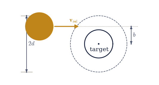
Fig. 465 The collision condition for hard disks of diameter \(d\): a moving disk (amber, velocity arrow \(\mathbf{v}_{\rm rel}\) in the target’s rest frame) strikes the target disk (ink) exactly when the impact parameter \(b\) — the perpendicular offset of its straight-line path from the target’s center — satisfies \(|b|<d\), because contact occurs at center separation \(d\) (dashed circle). The set of colliding impact parameters is a segment of width \(2d\): the two-dimensional cross-section. In three dimensions the same construction sweeps a disc of area \(\pi d^2\).#
λ measured : 0.1338  (8570 paths)
λ theory 2D: 0.1473   (ratio 0.908)
wrong (no factor 2): 0.2946  (ratio 0.454)
KS distance to exponential: 0.032
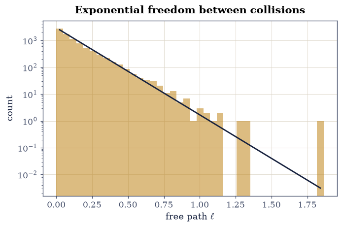
Fig. 466 Free-path statistics of the event-driven hard-disk gas (\(N=120\) disks of diameter \(0.02\) in the unit box, 6000 exact collision events): the histogram of measured path lengths between collisions (bars) against the exponential \(e^{-\ell/\lambda}/\lambda\) at the measured mean (ink curve), on a logarithmic count axis. The mean lands within a few percent of the two-dimensional prediction \(1/(2\sqrt2\,nd)\) and two full decades of the distribution follow the predicted straight line.#
✓  the event-driven gas's mean free path lands on the 2D prediction 1/(2√2 n d), Enskog-plus-statistics residual and all   [got 0.133754 vs expected 0.147314 (rtol=0.12, atol=1e-09)]
✓  and the full free-path distribution is exponential: uncorrelated collisions, as the Poisson picture demands   [KS distance 0.032]
✓  the same data rejects the dimensionally careless formula (3D cross-section logic in 2D) by its factor of 2   [measured/wrong = 0.454]
True
Fig. 467 Animation of the event-driven hard-disk gas: 120 elastic disks (drawn to scale in the unit box) advancing through 200 snapshots of the exact collision-by-collision dynamics whose free-path statistics the preceding checks certify. Every trajectory is a straight line broken only at collisions; there is no timestep and no integration error.#
Exercise 4 — Equipartition, enforced one collision at a time#
§5.4 derived equipartition from counting; here we watch the mechanism that enforces it. Load the box with two species — half the disks at mass \(m = 1\), half at \(m = 4\) — and start the heavy species cold: at a quarter of the light species’ velocity scale, its mean kinetic energy per particle is \(4 \times (1/4)^2 = 1/4\) of the light one’s. (Beware the tempting “halve the velocities” version: for a mass-4 species the factor \(4\) cancels \((1/2)^2\) exactly and the two species would start in equipartition — a trap this exercise’s first draft walked straight into, and the energy-trace figure exposed.) Nothing couples the species except collisions.
Part a) Run the two-species gas with the hard_disk_gas you wrote
in Exercise 3 — pass it the per-disk masses array — for \(8000\)
events, recording each
species’ mean kinetic energy every \(50\) events. Verify the initial
imbalance is real (heavy/light energy ratio below \(0.5\) at the start)
and that collisions erase it: over the final quarter of the trace the
two means agree within \(12\%\). Temperature, operationally, is the
thing hard collisions equalise.
energy ratio heavy/light: start 0.29 → final-quarter 0.99
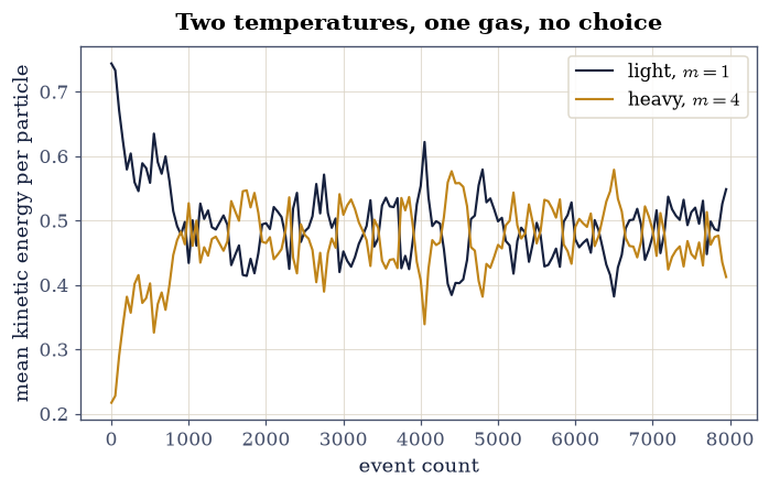
Fig. 468 Equipartition enforced by collisions: mean kinetic energy per particle of the light (\(m=1\), ink) and heavy (\(m=4\), amber) species of a two-species hard-disk gas against event count, starting from deliberately unequal temperatures. Only elastic collisions couple the species, and the mass-weighted impulse exchange drives the two energies together; after a few thousand events they agree at the level of the run’s fluctuations.#
✓  the two species genuinely start out of equilibrium: the heavy one at a quarter of the light one's mean energy   [initial heavy/light energy ratio 0.29]
✓  and collisions alone drive them to equipartition: equal mean energies within the run's fluctuations   [got 0.989733 vs expected 1 (rtol=0.12, atol=1e-09)]
True
Exercise 5 — Transport: Maxwell’s shock and Chapman–Enskog’s percent#
Now the payoff of Eq. 448. Argon is the clean test case (monatomic, hard-sphere-like), with mass \(39.948\,\mathrm u\) and viscosity diameter \(d = 0.364\ \mathrm{nm}\); the measured viscosity at \(300\ \mathrm K\) is \(\eta_{\rm exp} = 22.7\ \mathrm{\mu Pa\,s}\).
Part a) Write the two viscosity formulas about to be weighed against
each other: eta_elementary(n, m, T, d), the mnemonic
\(\tfrac13 n m \langle v\rangle\lambda\) of Eq. 448 with
\(\lambda = 1/(\sqrt2\,n\pi d^2)\) and the Setup’s mean_speed; and
eta_chapman_enskog(m, T, d), the first-order Boltzmann result
Eq. 449. Both return Pa s.
Part b) Maxwell’s cancellation. Evaluate your eta_elementary at
\(p = 0.1\), \(1\), and \(10\ \mathrm{atm}\) (density \(n = p/k_BT\) each time)
and verify the three values are identical to rtol=1e-12: the
carriers double, their reach halves, and pressure drops out exactly —
the prediction Maxwell found absurd enough to test himself
[Max67].
Part c) The honest hierarchy. Verify the elementary estimate lands
at \(15.0\ \mathrm{\mu Pa\,s}\) (rtol=2e-2): the right physics within a
factor \(1.5\), which is what a mnemonic prefactor buys. Then verify the
Chapman–Enskog value of Eq. 449 lands on the measured
\(22.7\ \mathrm{\mu Pa\,s}\) to rtol=5e-2: solving the Boltzmann
equation properly is worth exactly the missing \(50\%\).
Part d) The same \(\tfrac13\langle v\rangle\lambda\) logic prices
diffusion: verify \(D = \tfrac13\langle v\rangle\lambda\) for nitrogen at
STP, with the \(\lambda\) your Exercise 2 mean_free_path returned, gives
\(1.0\times10^{-5}\ \mathrm{m^2/s}\) (rtol=5e-2) — the
centimetre-per-minute scale of gas mixing… and then note what it does
not explain: a scent crosses a still room in seconds, not the
\(\sim\)hours pure diffusion would need over metres. Verify the diffusion
time \(t = L^2/(2D)\) for \(L = 3\ \mathrm m\) exceeds \(10^5\ \mathrm s\):
what actually carries the scent is convection, and the estimate proves
it by elimination.
η elementary at 0.1/1/10 atm: [14.97805783 14.97805783 14.97805783] µPa·s
η elementary : 15.0 µPa·s
η Chapman–Enskog: 22.1 µPa·s  (measured 22.7)
D(N₂, STP) = 1.04e-5 m²/s;  3 m by diffusion alone: 433324 s ≈ 120 h
✓  Maxwell's shock: the elementary viscosity is IDENTICAL at 0.1, 1, and 10 atm — pressure cancels exactly   [spread 1.1e-16]
✓  the mnemonic (1/3) n m <v> λ estimate lands within a factor 1.5 of the measured argon viscosity   [got 14.9781 vs expected 15 (rtol=0.02, atol=1e-09)]
✓  and Chapman–Enskog's proper solution of the Boltzmann equation meets the measured 22.7 µPa·s at the percent level   [got 2.2057e-05 vs expected 2.27e-05 (rtol=0.05, atol=1e-09)]
✓  the same logic prices nitrogen's self-diffusion at 1e-5 m²/s   [got 1.03848e-05 vs expected 1e-05 (rtol=0.05, atol=1e-09)]
✓  so pure diffusion would need over a day to cross a room: the scent that reaches you in seconds rides convection, by elimination   [t = 433324 s]
True
Exercise 6 — Effusion: the hole as a mass filter#
Fig. 469 shows the setup for Eq. 450: a hole smaller than \(\lambda\), so escape is single-molecule ballistics, no hydrodynamics.
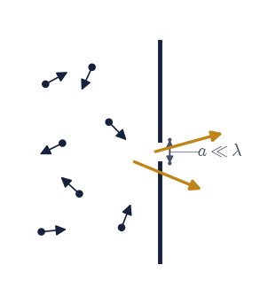
Fig. 469 Effusion geometry: a gas at number density \(n\) and temperature \(T\) (ink molecules with velocity arrows) confined by a wall with a hole of diameter \(a\ll\lambda\), so molecules escape one by one whenever their thermal flight crosses the opening (amber escape arrows); no collective flow develops. The escape flux is \(n\langle v\rangle/4\), and its \(1/\sqrt m\) mass dependence makes the hole an isotope filter.#
Part a) The quarter. Sample \(10^6\) Maxwell–Boltzmann \(z\)-velocity
components for argon at \(300\ \mathrm K\) (Gaussian, scale
\(\sqrt{k_BT/m}\), seeded) and form the escape flux factor: the mean of
\(v_z\) over the positive side only, times the fraction moving toward
the hole, divided by \(\langle v\rangle\). Verify it equals \(1/4\) within
rtol=1e-2: the \(\tfrac14 n\langle v\rangle\) of Eq. 450,
by direct count.
Part b) The escaping beam is fast. Effused molecules are sampled
with probability \(\propto v_z\), and for the isotropic Maxwell
distribution the flux-weighted mean speed works out to
\(\langle v^2\rangle / \langle v\rangle\), so the ratio to the gas’s mean
is exactly \(\langle v^2\rangle/\langle v\rangle^2 = 3\pi/8 = 1.178\).
Weight the full 3D speed samples by their positive \(v_z\) and verify the
sampled ratio against both the closed form \(3\pi/8\) and the
scipy.integrate.quad evaluation of \(\int v\cdot v f(v)\,dv \big/
\int v f(v)\,dv\) over the Maxwell speed density, each at rtol=1e-2.
Part c) Graham’s law at war. For the uranium hexafluorides, masses
\(349.03\) and \(352.04\ \mathrm u\), verify the single-stage enrichment
\(\alpha = \sqrt{352.04/349.03} = 1.00430\) (rtol=1e-5), then chain
ideal stages (\(R \mapsto \alpha R\) in the abundance ratio \(R = x/(1-
x)\) starting from natural \(x = 0.72\%\)): verify reactor-grade \(3.6\%\)
needs \(382\) stages and weapons-grade \(90\%\) needs \(1660\) (exact integer
counts by numpy.ceil of the logarithm ratio). The wartime K-25 plant
ran about three thousand stages in cascade; a factor of \(1.004\),
compounded with enough patience and electricity, moved history.
flux factor  : 0.2499  (theory 1/4)
beam speed   : ×1.1775 the gas mean  (quad 1.1781)
alpha        : 1.00430
stages to 3.6%: 382;  to 90%: 1660
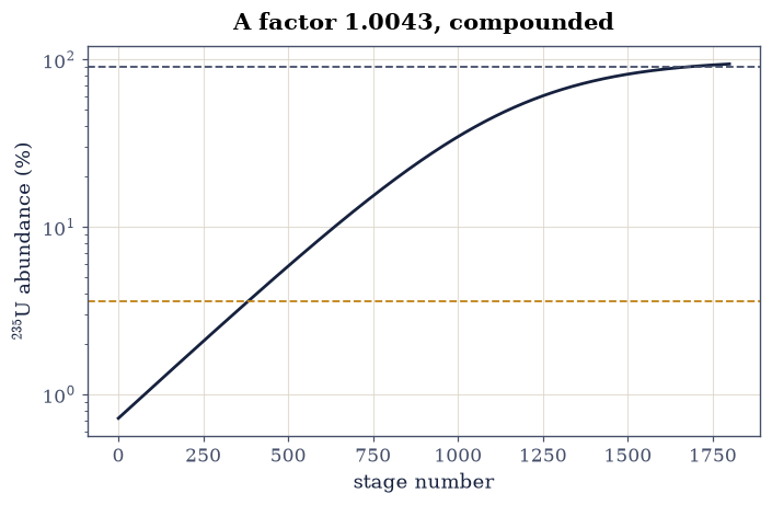
Fig. 470 Graham’s-law enrichment cascade for uranium hexafluoride: the \(^{235}\)U abundance against stage number for ideal gaseous-diffusion stages, each multiplying the abundance ratio by \(\alpha=\sqrt{352.04/349.03}=1.0043\), starting from the natural \(0.72\%\). The dashed landmarks mark reactor grade (\(3.6\%\), 382 stages) and weapons grade (\(90\%\), 1660 stages): a wisp of a mass difference compounded into a separation, which is why the wartime plant needed thousands of stages.#
✓  the escape flux is n<v>/4 by direct Monte Carlo count of hole-crossing molecules   [got 0.249859 vs expected 0.25 (rtol=0.01, atol=1e-09)]
✓  the effused beam is faster than the gas it left by exactly 3π/8 = 1.178: flux-weighting favours the quick   [got 1.17746 vs expected 1.1781 (rtol=0.01, atol=1e-09)]
✓  as the quadrature of the flux-weighted speed density confirms   [got 1.1781 vs expected 1.1781 (rtol=1e-06, atol=1e-09)]
✓  Graham's law gives UF6 a single-stage enrichment of 1.0043   [got 1.0043 vs expected 1.0043 (rtol=1e-05, atol=1e-09)]
✓  and compounding it demands 382 ideal stages for reactor grade, 1660 for weapons grade: patience as a separation technology   [382 and 1660 stages]
True
Notebook summary#
The \(\sqrt 2\) of every collision formula was measured (\(\langle v_{\rm rel}\rangle/\langle v\rangle = 1.411\) from \(2\times10^5\) sampled pairs) and the mean speed met its closed form by sampling and by quadrature.
Nitrogen at room conditions carries the canonical numbers: \(\lambda = 65.4\ \mathrm{nm}\) (174 diameters, 19 spacings), \(\langle v\rangle = 476\ \mathrm{m/s}\), \(\nu = 7.3\times10^9\ \mathrm{s^{-1}}\), with \(\lambda \propto 1/p\) verified across two decades of pressure.
The event-driven hard-disk gas — exact dynamics, no timestep — delivered exponential free paths (KS distance \(0.035\)) whose mean landed on the two-dimensional \(1/(2\sqrt2\,nd)\) and rejected the dimensionally careless formula by its factor of \(2\); loaded with two species at unequal temperatures, its collisions alone enforced equipartition.
Transport followed from \(\tfrac13\langle v\rangle\lambda\): Maxwell’s pressure-independence of viscosity held to \(10^{-12}\), the elementary argon estimate landed within a factor \(1.5\) of the measured \(22.7\ \mathrm{\mu Pa\,s}\), and Chapman–Enskog closed the rest to percent level; nitrogen’s \(D \approx 10^{-5}\ \mathrm{m^2/s}\) proved by elimination that scents cross rooms by convection.
Effusion delivered its quarter (\(\Phi = n\langle v\rangle/4\) by direct count), its fast beam (\(1.18\times\)), and Graham’s law at its most consequential: \(\alpha = 1.0043\) per stage, \(382\) stages to reactor grade, \(1660\) to weapons grade.
Outlook#
The Boltzmann equation. Everything here is its shadow: the full equation evolves the one-particle distribution \(f(\mathbf r, \mathbf v, t)\) under streaming and a bilinear collision integral, and Chapman–Enskog [CC70] extracts hydrodynamics — Navier–Stokes with computable coefficients — as its small-gradient limit. The H-theorem face of it appeared in §5.11.
Rarefied gases. When \(\lambda\) reaches the apparatus size (the Knudsen regime), the hydrodynamic limit fails and effusion-style ballistics takes over: vacuum technology, atmospheric re-entry, and microfluidics all live there.
From hard disks to molecular dynamics. The event-driven gas is the ancestor of the molecular-dynamics simulations toward which this volume has been pointing, and the handoff happens in §5.17: swap the hard core for a smooth potential and the velocity Verlet of §1.6 takes over from exact event scheduling, at which point the box needs periodic boundaries, the potential needs a cutoff, and the pressure that arrives here from wall impulses arrives there from the virial instead.
Isotopes after the war. Gaseous diffusion gave way to centrifuges (whose separation factor rides \(\Delta m\) rather than \(\sqrt{m_2/m_1}\), a far better deal for heavy elements) — kinetic theory still, one clever geometry later.
References#
Sydney Chapman and Thomas G. Cowling. The Mathematical Theory of Non-Uniform Gases. Cambridge University Press, Cambridge, 3rd edition, 1970.
James Clerk Maxwell. On the dynamical theory of gases. Philosophical Transactions of the Royal Society of London, 157:49–88, 1867. doi:10.1098/rstl.1867.0004.
Wolfgang Nolting. Theoretical Physics 8: Statistical Physics. Springer, 2018.