


3.17 Crystal Optics: Birefringence and the Wave Surface#
Notebook overview#
§3.16 ended one step short of the optics. It established that a crystal answers a field with a tensor, that diagonalizing that tensor finds the material’s own axes, and that everywhere off those axes the displacement \(\mathbf D\) points somewhere the field \(\mathbf E\) does not, by an angle that reached \(15.83^\circ\) for the model crystal and \(6.26^\circ\) for calcite. Then it stopped, and named what comes next as a horizon without giving it a number. This is that notebook.
The optics follows from one extra fact, which the electrostatics of
§3.16 had no occasion to use: a plane wave is
transverse in \(\mathbf D\), not in \(\mathbf E\). Gauss’s law in a source-free dielectric
says \(\nabla\cdot\mathbf D=0\), so \(\mathbf D\) lies in the plane perpendicular to the
propagation direction, while \(\mathbf E=\boldsymbol\varepsilon^{-1}\mathbf D/\varepsilon_0\)
generally does not. Combine that with the wave equation of
§3.8 and the whole subject drops out. Each propagation direction
admits exactly two waves, with two different refractive indices and two orthogonal
polarizations, and finding them is a two-by-two real symmetric eigenvalue problem that
numpy.linalg.eigh solves in one line. That reduction is the notebook’s engine, and
the classical statement of it is Fresnel’s equation of wave normals, which we
derive, put into a form a computer can actually solve, and then check the engine
against.
Three consequences occupy the rest. In a uniaxial crystal one of the two waves is blind to direction, its index sitting at \(n_o\) no matter where the wave goes, while the other traces an ellipse from \(n_o\) to \(n_e\): those are the ordinary and extraordinary rays, and calcite splits a beam into them. Then walk-off, which is the whole point of the connection to §3.16: the Poynting vector \(\mathbf E\times\mathbf H\) is perpendicular to \(\mathbf E\), the wave normal is perpendicular to \(\mathbf D\), and since those two are not parallel neither are these. The energy travels at an angle to its own wavefront. The angle is the same angle between \(\mathbf D\) and \(\mathbf E\) that §3.16 measured, and its maximum for calcite comes out \(6.26^\circ\) again, from a formula with the identical shape. A ray in calcite goes somewhere its wave normal does not, and a centimetre of the crystal turns that into a millimetre of doubled image. Finally the two indices per direction, plotted as a radius, make a two-sheeted surface whose sheets touch at exactly one place, the optic axis, and whose ray counterpart is the surface Huygens drew in 1690.
The last exercise takes the phase difference the two waves accumulate and cuts a wave plate out of it: a slab thick enough to retard one polarization by a quarter of a cycle relative to the other turns linear light into circular, and a half-cycle slab reflects the polarization about the plate’s own axis. We do that through the physical phase difference and the field it produces, tracing the real electric vector over one optical cycle and measuring the ellipse it draws.
Everything is SI, the permittivity tensor is the dimensionless relative one of §3.16, and the medium is taken non-magnetic (\(\mu=\mu_0\)), lossless and non-absorbing, so \(\boldsymbol\varepsilon\) is real and symmetric. Dispersion, which §3.15 built in full, is switched off here: every index is quoted at the sodium D line, \(\lambda=589.3\,\)nm, and held fixed. The worked material is calcite, through the same measured indices §3.16 used, \(n_o=1.6584\) and \(n_e=1.4864\); the model biaxial crystal of that notebook, \(\boldsymbol\varepsilon=\mathrm{diag}(2.40,3.00,4.20)\), returns for the final exercise. Plane waves are written \(e^{i(\mathbf k\cdot\mathbf r-\omega t)}\), as in §3.15.
How to read the checks. Each exercise ends with a
validatecall against something the computation did not assume: a closed form derived in the statement, the residual of the full three-dimensional wave equation, an index recovered from a rotated sample, a measured ellipse against its analytic ellipticity. A validation compares a result to an expected fact, so a ✗ does not by itself mean the answer is wrong: it may be a genuine error, a different-but-valid convention (an eigenvector sign, an axis ordering, a branch), or too tight a tolerance. Treat a ✗ as a prompt to locate the discrepancy. Passing is strong evidence, not proof. Two structural facts below — that \(\mathbf D\) comes out transverse and that the two polarizations come out orthogonal — are guaranteed by the way the engine is built, so they are reported rather than checked, and the validation prose says so where they appear.
Scope. A working review, not a full course. Born and Wolf [BW99] (ch. 15) is the standard account and the source of the conventions used here; see also Jackson [Jac98] (ch. 7), Griffiths [Gri17] (ch. 9), Nolting, Theoretical Physics 3 [Nol16], and Yariv and Yeh, Optical Waves in Crystals, which develops the same material with the engineering conventions.
Theory in brief#
What a plane wave in a crystal is allowed to be#
Take Maxwell’s equations in a source-free, non-magnetic, anisotropic dielectric and insert a monochromatic plane wave, \(\mathbf E,\mathbf D,\mathbf H\propto e^{i(\mathbf k\cdot\mathbf r-\omega t)}\) with \(\mathbf k=(\omega n/c)\,\hat{\mathbf s}\), so that \(\hat{\mathbf s}\) is the wave normal and \(n\) the refractive index for that direction. The two curl equations become \(\mathbf k\times\mathbf E=\omega\mu_0\mathbf H\) and \(\mathbf k\times\mathbf H=-\omega\mathbf D\); eliminating \(\mathbf H\) between them, exactly as §3.8 eliminated \(\mathbf B\) to reach the vacuum wave equation, gives
The bracket is the part of \(\mathbf E\) perpendicular to \(\hat{\mathbf s}\). In an isotropic medium \(\boldsymbol\varepsilon=\varepsilon\mathsf 1\) and Eq. 299 forces \(\hat{\mathbf s}\cdot\mathbf E=0\) and \(n^2=\varepsilon\): one index, one wave, transverse in \(\mathbf E\). In a crystal neither conclusion survives. What does survive is that the left side equals \(\mathbf D/\varepsilon_0\) and the right side is manifestly perpendicular to \(\hat{\mathbf s}\), so
which is \(\nabla\cdot\mathbf D=0\) read off a plane wave. The displacement is transverse; the field is not. Everything in this notebook is a consequence of that one sentence.
Two waves per direction, from a two-by-two eigenproblem#
Because \(\mathbf D\) is the transverse object, it is the better unknown. Write \(\mathbf E=\boldsymbol\eta\cdot\mathbf D/\varepsilon_0\) with \(\boldsymbol\eta=\boldsymbol\varepsilon^{-1}\) the impermeability tensor that §3.16 introduced as the object whose quadric surface is the index ellipsoid. Substituting into Eq. 299 and projecting onto the plane perpendicular to \(\hat{\mathbf s}\) with \(\mathsf P=\mathsf 1-\hat{\mathbf s}\hat{\mathbf s}^{\mathsf T}\) turns the whole thing into
That is an eigenvalue problem for a real symmetric operator acting on a two-dimensional space, the plane perpendicular to \(\hat{\mathbf s}\). Pick any orthonormal pair \((\hat{\mathbf u},\hat{\mathbf v})\) spanning that plane, form the \(2\times2\) matrix \(M_{ab}=\hat{\mathbf u}_a\cdot\boldsymbol\eta\cdot\hat{\mathbf u}_b\), and the spectral theorem of §0.5 delivers two eigenvalues \(1/n^2\) and two orthogonal eigenvectors. A direction through a crystal admits exactly two waves. Geometrically the matrix \(M\) is the index ellipsoid of §3.16 cut by the plane through its centre perpendicular to \(\hat{\mathbf s}\): the two semi-axes of that elliptical section are the two indices, and their directions are the two allowed \(\mathbf D\) polarizations. Reading the indicatrix section by section, which §3.16 named as the thing to do with it and did not do, is what Eq. 300 does numerically.
Fresnel’s equation of wave normals#
The classical form of the same statement is a scalar equation, obtained by writing Eq. 299 in the crystal’s principal axes and demanding that the resulting \(3\times3\) homogeneous system have a non-trivial solution. Expanding that determinant and dividing through by \(\prod_i(n^{-2}-n_i^{-2})\) gives Fresnel’s equation of wave normals,
with \(s_i\) the components of \(\hat{\mathbf s}\) along the principal axes. Born and Wolf [BW99] (§15.2) derive it in full. It is the form printed in every textbook, and it is the wrong form to hand a root-finder, because the division that produced it is illegal whenever a root coincides with one of the \(n_i\) — which is exactly what happens in a uniaxial crystal. Undoing the division restores a plain quadratic in \(u=1/n^2\),
whose two roots are the two indices in every case, degenerate or not. Exercise 2 solves
Eq. 302 with numpy.roots and watches Eq. 301 diverge
where its own root should be.
Uniaxial crystals: ordinary and extraordinary#
A crystal with two equal principal permittivities is uniaxial, the odd direction being the optic axis \(\hat{\mathbf a}\). Write the pair as \(n_o\) (ordinary) and the odd one as \(n_e\) (extraordinary), and let \(\theta\) be the angle between the wave normal and the optic axis. Then Eq. 302 factors, and the two roots are
The ordinary wave is polarized with \(\mathbf D\) perpendicular to the plane containing \(\hat{\mathbf s}\) and \(\hat{\mathbf a}\), so it never sees the odd principal value at all and its index is a constant. The extraordinary wave is polarized in that plane and its index runs from \(n_o\) on the axis to \(n_e\) at right angles to it. Calcite has \(n_e<n_o\) and is called negative; quartz has \(n_e>n_o\) and is positive.
Walk-off: where the energy actually goes#
The energy flux is the Poynting vector of §3.8, \(\mathbf S=\mathbf E\times\mathbf H\), and with \(\mathbf H\propto\hat{\mathbf s}\times\mathbf E\) from the curl equation above,
Now count perpendiculars. \(\mathbf D\perp\hat{\mathbf s}\) and \(\mathbf E\perp\mathbf S\), while \(\mathbf H\) is perpendicular to all four, so \(\mathbf D\), \(\mathbf E\), \(\hat{\mathbf s}\) and \(\mathbf S\) are coplanar and the pair \((\mathbf E,\mathbf S)\) is the pair \((\mathbf D,\hat{\mathbf s})\) rotated rigidly through one angle. The angle between the ray and the wave normal equals the angle between \(\mathbf E\) and \(\mathbf D\). That angle is precisely the quantity §3.16 measured over the sphere of field directions, and here it acquires a name, the walk-off angle \(\rho\), and a job: it is how far the beam drifts sideways per unit of propagation. For a uniaxial crystal, with \(\theta\) again the angle from the optic axis,
which vanishes on the optic axis and at right angles to it, and is largest in between:
Compare Eq. 306 with the maximum \(\mathbf D\)–\(\mathbf E\) angle of §3.16, \(\tan\alpha_{\max}=(\varepsilon_3-\varepsilon_1) /2\sqrt{\varepsilon_1\varepsilon_3}\). With \(\varepsilon_i=n_i^2\) the two are the same formula. Exercise 8 of §3.16 computed this number for calcite and got \(6.26^\circ\) from a crystal turning on a turntable; the same \(6.26^\circ\) is about to reappear as the angle by which a beam of light leaves its own wavefront behind.
Two surfaces#
Plotting the index as a radius, \(n(\hat{\mathbf s})\,\hat{\mathbf s}\), sweeps out the index surface (or wave-vector surface), which has two sheets because there are two indices per direction. For a uniaxial crystal the ordinary sheet is a sphere of radius \(n_o\) and the extraordinary sheet is a spheroid; in the plane containing the optic axis \(\hat{\mathbf e}_3\), with \(x\) measured perpendicular to it,
Its semi-axes are the opposite way round from the index ellipsoid of §3.16, which had semi-axis \(n_e\) along the optic axis. The two sheets meet where \(n^{(e)}=n_o\), which by Eq. 303 is \(\theta=0\) alone: the optic axis is the single direction in a uniaxial crystal that does not split light. The wave surface (or ray surface) is the same information carried by the rays: the locus reached in unit time by energy leaving a point source, which is Huygens’ secondary wavelet. Its extraordinary sheet is again a spheroid, but with the axes exchanged once more,
and the ray speed along a ray tilted by \(\rho\) from its wave normal is \(v_{\rm ray}=c/(n\cos\rho)\), since the wavefront advances at \(c/n\) along \(\hat{\mathbf s}\) and the ray covers the hypotenuse.
Retardance, and the wave plate#
Send light through a slab of thickness \(d\) cut so that the optic axis lies in the face. The wave normal is then perpendicular to the optic axis, the two allowed polarizations have indices exactly \(n_o\) and \(n_e\), and after the slab they differ in phase by
A quarter-wave plate has \(\Delta\phi=\pi/2\) and a half-wave plate \(\Delta\phi=\pi\). What each does to a polarization state is then a question about the real field: if the incoming light is linearly polarized at azimuth \(\psi\) to the plate’s axes, the field leaving the plate is \(\mathbf E(t)\propto(\cos\psi\cos\omega t,\;\sin\psi\cos(\omega t-\Delta\phi))\), whose tip traces an ellipse. Its ellipticity angle \(\chi\), defined by \(\tan\chi=B/A\) from the semi-axes, satisfies
so a quarter-wave plate at \(\psi=45^\circ\) gives \(\chi=45^\circ\), a circle. Exercise 7 traces the ellipse and measures it rather than asserting this.
Biaxial crystals, in one paragraph#
When all three principal values differ, the section of the indicatrix perpendicular to \(\hat{\mathbf s}\) is circular for two directions rather than one, and the crystal is called biaxial. Both lie in the plane of the largest and smallest principal indices, at an angle \(\beta\) from the largest-index axis given by
which Exercise 8 derives in three lines and then locates numerically. That is as far as this notebook goes into the biaxial case, and the last exercise says why.
Setup#
Data and one set of restated instruments. The data are the two measured refractive
indices of calcite and of quartz at the sodium D line, that wavelength itself, the three
principal relative permittivities of the model biaxial crystal that
§3.16 worked with, the speed of light from
scipy.constants, and the series palette. The instruments are the three helpers the
reader wrote from scratch in §3.16 — the rotation
matrix, the rank-2 transformation law and the angle between \(\mathbf D\) and \(\mathbf E\)
— restated here so a laboratory-frame crystal can be built without rebuilding machinery
already earned. Nothing this notebook is about is pre-built: the transverse eigenproblem
Eq. 300, the polynomial form Eq. 302 of Fresnel’s
equation, the Poynting construction Eq. 304, the two surfaces and the
wave-plate field are all assembled in the exercises. Nothing here is stochastic.
The Setup below holds this notebook’s data and instruments — nothing you are asked to build. It is collapsed so the building stays yours; expand it whenever you want the details.
Exercise 1 — Two waves per direction (worked)#
Pick a direction through a crystal and ask what a plane wave travelling that way is allowed to look like. In vacuum, or in glass, the answer is a one-liner: the field is perpendicular to the propagation direction, any polarization in that plane will do, and the index is the same number for all of them. In a crystal the algebra of Eq. 299 gives a different answer, and the reason is the observation that opened the notebook: it is \(\mathbf D\), not \(\mathbf E\), that has to lie in the transverse plane (Fig. 325).
Because of that, the natural unknown is \(\mathbf D\), and the natural operator is the impermeability \(\boldsymbol\eta=\boldsymbol\varepsilon^{-1}\) of §3.16. Restricting Eq. 300 to the plane perpendicular to \(\hat{\mathbf s}\) leaves a \(2\times2\) real symmetric matrix, whose two eigenvalues are \(1/n^2\) for the two permitted waves and whose two eigenvectors are their \(\mathbf D\) polarizations. This is the notebook’s engine; everything after it is a question asked of this one function.
The specimen is calcite, whose relative permittivity tensor in its own axes is \(\boldsymbol\varepsilon_c=\mathrm{diag}(n_o^2,\,n_o^2,\,n_e^2)= \mathrm{diag}(2.750291,\,2.750291,\,2.209385)\) built from the measured \(n_o=1.6584\) and \(n_e=1.4864\), with the optic axis along \(\hat{\mathbf e}_3\). The worked direction is \(\hat{\mathbf s}=(\sin30^\circ,\,0,\,\cos30^\circ)\), thirty degrees from the optic axis in the \(\hat{\mathbf e}_1\)–\(\hat{\mathbf e}_3\) plane.
Part a) Write wave_normal_modes(eps, s_hat) returning the two indices and the two
\(\mathbf D\) directions for one wave normal. Normalize s_hat with
numpy.linalg.norm; form \(\boldsymbol\eta\) with numpy.linalg.inv; build an
orthonormal pair spanning the transverse plane by crossing s_hat with whichever of
\(\hat{\mathbf e}_3\) or \(\hat{\mathbf e}_1\) is less nearly parallel to it (numpy.cross,
then normalize, then cross again); assemble the \(2\times2\) matrix as the contraction
numpy.einsum("ai,ij,bj->ab", basis, eta, basis); symmetrize it as 0.5 * (M + M.T)
against round-off; diagonalize with numpy.linalg.eigh (not numpy.linalg.eig —
the matrix is real symmetric, and eigh alone guarantees real eigenvalues and an
orthonormal eigenbasis); return 1 / numpy.sqrt(eigenvalues) and the two eigenvectors
expressed back in three dimensions as coefficients.T @ basis.
Write this one yourself — the implementation is the lesson.
Part b) Write the one-line helper wave_normal(theta) returning
\((\sin\theta,0,\cos\theta)\), the wave normal at angle \(\theta\) from the optic axis in
the \(\hat{\mathbf e}_1\)–\(\hat{\mathbf e}_3\) plane, and evaluate the engine at
\(\theta=30^\circ\) for calcite. Print both indices and both polarizations, and report
\(\max|\mathbf D_k\cdot\hat{\mathbf s}|\) and \(|\mathbf D_1\cdot\mathbf D_2|\).
Part c) Certify the reduction against the equation it came from. For each mode form
\(\mathbf E=\boldsymbol\eta\cdot\mathbf D\) with numpy.linalg.solve(eps, D) (a linear
solve, not an explicit inverse), and evaluate the residual of the full
three-dimensional Eq. 299,
numpy.max(numpy.abs(eps @ E - n**2 * (E - s_hat * numpy.dot(s_hat, E)))). Nothing in
the two-by-two construction guaranteed that the third component would come out right, so
this is the check that the reduction is faithful.
Part d) Compare the two indices with the uniaxial closed forms Eq. 303: \(n_o=1.6584\) exactly, and \(n^{(e)}(30^\circ)=[\cos^2 30^\circ/n_o^2+\sin^2 30^\circ/n_e^2]^{-1/2}\). Report the splitting \(|n^{(o)}-n^{(e)}|\) as well: it is what makes the direction birefringent at all.
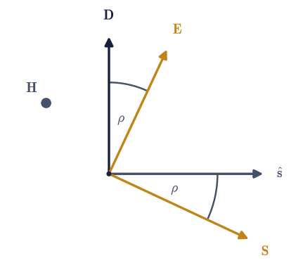
Fig. 325 The four vectors of a plane wave in a crystal, all lying in one plane because the magnetic field \(\mathbf H\) is perpendicular to every one of them and points out of the page. The wave normal \(\hat{\mathbf s}\) fixes the direction in which the phase advances and the displacement \(\mathbf D\) is perpendicular to it, as \(\nabla\cdot\mathbf D = 0\) requires. The electric field \(\mathbf E = \boldsymbol\eta\cdot\mathbf D/\varepsilon_0\) is tilted away from \(\mathbf D\) by an angle \(\rho\) because the impermeability tensor multiplies its components by different numbers, and the energy flux \(\mathbf S = \mathbf E\times\mathbf H\) is perpendicular to \(\mathbf E\) and therefore tilted away from \(\hat{\mathbf s}\) by the same \(\rho\). The tilt is drawn at \(25^\circ\) for legibility; in calcite it never exceeds \(6.26^\circ\).#
calcite tensor diag: [2.750291 2.750291 2.209385]
two indices at θ = 30°: [1.6584      1.609865351]
their D polarizations (rows):
[[ 0.        1.        0.      ]
 [-0.866025  0.        0.5     ]]
max |D·ŝ| = 7.44e-18 (transverse by construction)
|D₁·D₂| = 0.00e+00 (orthogonal by construction)
residual of eq-co-wave, both modes: [3.33e-16 1.11e-16]
closed forms: n_o = 1.658400000, n_e(30°) = 1.609865351
birefringent splitting at θ = 30°: Δn = 0.048535
Validation 1#
Two things are checked, and one is reported without being checked. The residual of Eq. 299 is the substantive test: the engine solved a two-dimensional problem, and nothing in that construction forced the third component of the full equation to balance, so a residual at machine precision says the reduction is faithful. The comparison with Eq. 303 is independent in a different sense: those closed forms never entered the computation. That the splitting is not zero matters too, since every later exercise would be vacuous on a direction that happened not to split. The transversality and orthogonality figures printed above are guaranteed by the construction and would remain small even if the physics were wrong, so they are not validated here.
✓  both solved modes satisfy the full three-dimensional wave equation eq-co-wave   [max|Δ| = 3.33067e-16 (rtol=0, atol=1e-14)]
✓  the two indices are n_o = 1.6584 and n_e(30°) = 1.609865 from eq-co-uniaxial   [max|Δ| = 2.22045e-16 (rtol=1e-12, atol=1e-09)]
✓  the direction is genuinely birefringent, so the two-wave statement is not vacuous   [Δn = 0.048535 at θ = 30°]
True
Exercise 2 — Fresnel’s equation of wave normals (student)#
The engine of Exercise 1 is a modern reduction. The classical statement of the same content is a single scalar equation, and it is worth having both, because they fail in different places and each catches the other’s mistakes.
Its derivation is short. Write Eq. 299 in the crystal’s principal axes, where \(\boldsymbol\varepsilon\) is diagonal, and it becomes three coupled equations for the three components of \(\mathbf E\); a homogeneous linear system has a non-trivial solution only when its determinant vanishes, and expanding that \(3\times3\) determinant, then dividing by \(\prod_i(n^{-2}-n_i^{-2})\), gives Fresnel’s equation of wave normals Eq. 301. Born and Wolf [BW99] (§15.2) carry the expansion out in full.
The division is where the trouble is. It is legal only when no root of the equation
coincides with a principal index, and in a uniaxial crystal the ordinary root sits
exactly on \(n_o\), which is a pole of two of the three terms in Eq. 301.
The textbook form therefore cannot see its own root, and no bracketing root-finder such
as scipy.optimize.brentq will locate it. Undoing the division restores
Eq. 302, a plain quadratic in \(u=1/n^2\) whose two roots are always the
two indices. That distinction between an equation and a computable equation is the
lesson of this exercise as much as the physics is.
Part a) Write fresnel_coefficients(eps, s_hat) returning the three coefficients
\([c_2,c_1,c_0]\) of \(F(u)=c_2u^2+c_1u+c_0\) from Eq. 302, in the order
numpy.roots expects. Take \(u_i=1/\varepsilon_i\) from numpy.diag(eps), normalize the
squared components \(s_i^2\) so they sum to one, and accumulate the three products
\(s_i^2(u-u_j)(u-u_k)\) term by term into an explicit numpy array of three entries. This
form assumes eps is given in the crystal’s principal axes; say so in the docstring,
because Part d turns on it.
Part b) Solve it for calcite along
\(\hat{\mathbf s}=(\sin30^\circ,0,\cos30^\circ)\) with numpy.roots, convert the two
roots with \(n=1/\sqrt{u}\), and compare with the pair wave_normal_modes returned in
Exercise 1. Then sweep \(\theta\) over 181 angles spaced linearly on \([0,\pi/2]\) with
numpy.linspace, using the wave_normal(theta) helper of Exercise 1, and report
numpy.max of the absolute difference between the two routes twice: once over the whole
sweep, and once over the directions at least \(5^\circ\) from the optic axis.
The two numbers will not be the same, and the gap between them is the point of the part.
numpy.roots works by building the companion matrix of the polynomial and
eigendecomposing it, and a polynomial with two nearly coincident roots is
ill-conditioned: a perturbation \(\epsilon\) in the coefficients moves a double root by
order \(\sqrt\epsilon\), so about half the available digits are lost. Near the optic axis
the two waves are nearly degenerate, which is exactly the regime where the polynomial
route is weakest. The symmetric eigenproblem has no such trouble, because for a real
symmetric matrix the eigenvalue error is bounded by the perturbation of the matrix
itself, with no gap in the denominator, which is the Weyl bound behind the reliability of
eigh in §0.5. Report the disagreement at
\(\theta=0.5^\circ\) alongside the index splitting there, so the loss can be seen against
the degeneracy that causes it.
Part c) Watch the textbook form fail. Evaluate \(\sum_i s_i^2/(u-u_i)\) at \(u=u_o+\delta\) for \(\delta=10^{-3},10^{-5},10^{-7}\), where \(u_o=1/n_o^2\) is the ordinary root itself. Instead of approaching zero the sum grows like \(1/\delta\); multiply each value by its own \(\delta\) and watch the product approach \(s_1^2+s_2^2=1-s_3^2=0.25\), which identifies the divergence as a simple pole with exactly the residue the algebra predicts. It approaches it rather than sitting on it, because the remaining term \(s_3^2/(u-u_e)\) is finite at \(u_o\) and contributes an error linear in \(\delta\); report the three errors and the ratios between them, which should be \(100\) for each factor-of-\(100\) reduction in \(\delta\). Grading the limit against \(0.25\) without allowing for that term would be grading the leading behaviour against the whole answer.
Part d) The eigenproblem does not care about the frame, and the polynomial does.
Build \(\mathsf R\) for \(\hat{\mathbf n}\propto(1,2,3)\) and \(\theta=37^\circ\) with the
rotation_matrix of the Setup, rotate the calcite tensor with transform_tensor, rotate
\(\hat{\mathbf s}\) with the matrix product R @ s_hat, and confirm with
numpy.allclose that wave_normal_modes returns the same two indices as in Part b.
Refractive index is a scalar, so nothing else was ever possible, and the check is a test
of Eq. 300 and of the transformation law together.
Fresnel polynomial roots at θ = 30°: [1.609865351 1.6584     ]
engine of Exercise 1:                [1.609865351 1.6584     ]
largest disagreement over all 181 directions: 5.32e-12
largest disagreement at least 5° from the optic axis: 5.86e-14
the worst case is θ = 0.5°, where the two roots are only 1.55e-05 apart
eq-co-fresnel evaluated just above the ordinary root u_o:
   δ = 1e-03:  sum =   2.4148e+02,  sum × δ = 0.24147889,  error 8.52e-03
   δ = 1e-05:  sum =   2.4992e+04,  sum × δ = 0.24991574,  error 8.43e-05
   δ = 1e-07:  sum =   2.5000e+06,  sum × δ = 0.24999916,  error 8.43e-07
expected residue s₁² + s₂² = 1 − s₃² = 0.250000
error ratios between successive δ: [101.125 100.01 ]
same wave, laboratory frame: [1.609865351366 1.6584        ]
same wave, crystal frame:    [1.609865351366 1.6584        ]
Validation 2#
The first check is a genuine cross-method comparison: a \(2\times2\) symmetric eigenproblem on one side and the roots of a quadratic assembled from a different expression on the other, agreeing to \(10^{-13}\) at every direction that is not nearly degenerate. The second is the conditioning statement, and it is written as a band, with a floor as well as a ceiling: near the optic axis the polynomial route must be worse than it is elsewhere, by a margin large enough not to be an accident, and still far better than the physical splitting it is trying to resolve. A check with only one side would pass whether or not the effect was there. The third turns the failure of Eq. 301 into a quantitative statement rather than a warning: multiplied by \(\delta\), the diverging sum approaches the residue the algebra predicts, which is what “simple pole” means, and it approaches it at the first-order rate the one finite remaining term dictates. Checking the rate as well as the limit is what makes the pair a test of the expansion rather than of a single number. The last says the two indices are scalars.
✓  away from the optic axis the two routes to Fresnel's equation agree to 10⁻¹³   [max|Δ| = 5.86198e-14 (rtol=0, atol=1e-13)]
✓  and near it the companion-matrix route loses about half its digits, as a near-double root must   [worst 5.32e-12 at a splitting of 1.55e-05]
✓  the ordinary root is a simple pole of eq-co-fresnel, with residue s₁² + s₂² = 0.25   [got 0.249999 vs expected 0.25 (rtol=1e-05, atol=1e-09)]
✓  and the approach to it is linear in δ, as the one finite remaining term requires   [max|Δ| = 1.12479 (rtol=0.02, atol=1e-09)]
✓  so the textbook form never vanishes near its own root and no bracketing solver can find it   [smallest value reached: 2.415e+02]
✓  both indices survive rotating tensor and wave normal together: n is a scalar   [max|Δ| = 4.44089e-16 (rtol=0, atol=1e-13)]
True
Exercise 3 — The ordinary index that ignores direction (student)#
Calcite is uniaxial: two of its three principal permittivities coincide, so its index ellipsoid is a spheroid and every direction in the equatorial plane is equivalent, which is the degeneracy §3.16 demonstrated by handing an eigensolver an arbitrary pair of axes inside that plane. The optical consequence is the one the words ordinary and extraordinary record. One of the two waves has its \(\mathbf D\) perpendicular to the plane containing the wave normal and the optic axis, so it lies wholly in the equatorial plane where the crystal has nothing to distinguish one direction from another, and its index is \(n_o\) no matter where the wave is heading. That is the ordinary wave, and it obeys ordinary optics. The other has \(\mathbf D\) in that plane, samples both principal values, and its index runs from \(n_o\) to \(n_e\) as the wave normal turns away from the axis, following the ellipse of Eq. 303. That is the extraordinary wave, and it is the one that misbehaves.
Sorting the two eigenvalues by size would be the wrong way to tell them apart, because it labels by an accident of magnitude rather than by physics: in a positive crystal like quartz the ordering is reversed, and at the optic axis there is no ordering at all. Label them instead by the property that defines them, \(\mathbf D\cdot\hat{\mathbf a}=0\) for the ordinary wave, where \(\hat{\mathbf a}=\hat{\mathbf e}_3\) is the optic axis.
Part a) Sweep \(\theta\) over 2001 angles spaced linearly on \([0,\pi/2]\) with
numpy.linspace, and at each one call the wave_normal_modes and wave_normal
built in Exercise 1 on calcite,
\(\boldsymbol\varepsilon_c=\mathrm{diag}(2.750291,2.750291,2.209385)\). Identify the
ordinary mode at each direction as the one minimizing \(|\mathbf D\cdot\hat{\mathbf e}_3|\)
with numpy.argmin, and collect the two index arrays.
Part b) Report numpy.ptp of the ordinary index over the whole sweep. It is a
theorem that this vanishes, and the theorem is being tested against a \(2\times2\) matrix
whose entries change at every one of the 2001 directions.
Part c) Compare the extraordinary index with Eq. 303 over the same sweep, and report its two endpoints: \(n^{(e)}(0)\) must be \(n_o=1.6584\), where the two waves are indistinguishable, and \(n^{(e)}(90^\circ)\) must be \(n_e=1.4864\).
Part d) Confirm the labelling was physical rather than lucky, and do it in a frame
where the answer cannot be arranged. In the crystal frame the transverse basis the engine
builds happens to contain \(\pm\hat{\mathbf e}_2\) exactly, because the wave normal stays
in the \(\hat{\mathbf e}_1\)–\(\hat{\mathbf e}_3\) plane, so
\(|\mathbf D_{\rm ord}\cdot\hat{\mathbf e}_3|\) comes out identically zero partly by
construction; report it, and then do the test properly. Rotate the tensor and every wave
normal of the sweep by the \(\mathsf R\) of Exercise 2 with transform_tensor and the
matrix product R @ s, so that the rotated optic axis R[:, 2] lies along no basis
vector the engine will build, and report
numpy.max(numpy.abs(D_ordinary_rotated @ axis_rotated)) over the directions with
\(\theta\ge1^\circ\). Below that the two indices are within \(10^{-4}\) of each other and the
polarizations are not defined at all, so the quantity is meaningless there rather than
wrong.
Part e) Plot both indices against \(\theta\) in degrees on one pair of axes, with the two limiting values marked, and beside it \(|\mathbf D\cdot\hat{\mathbf e}_3|\) for both modes, which is the labelling made visible (Fig. 326).
ordinary index over 2001 directions: 1.658400000000 ... 1.658400000000
total variation numpy.ptp(n_ord) = 0.00e+00
extraordinary index vs eq-co-uniaxial: max|Δ| = 6.66e-16
endpoints: n_e(0°) = 1.6584000000, n_e(90°) = 1.4864000000
max |D_ord · ê₃| for θ ≥ 1°, crystal frame: 0.00e+00
   (partly structural: the engine's transverse basis contains ±ê₂ in this geometry)
max |D_ord · â| for θ ≥ 1° in a rotated frame: 4.42e-14
Validation 3#
The first check is the exercise’s whole point, and it is a real one: the engine solves a different \(2\times2\) matrix at every direction, and the ordinary eigenvalue coming back identical to the last bit is a statement about calcite, not about the code. The second grades the extraordinary branch against a closed form the computation never used. The third says the labelling was earned. It is deliberately run on a rotated crystal: in the crystal frame the engine happens to build \(\pm\hat{\mathbf e}_2\) as one of its two transverse basis vectors, so the same quantity would come out identically zero there whether or not the eigenproblem had found anything, and a check that cannot fail is not a check. Turned by \(37^\circ\) about \(\hat{\mathbf n}\propto(1,2,3)\) the optic axis lies along nothing the construction produces, and the eigensolver has to find the ordinary polarization on its own. The result is no longer an exact zero but a round-off one, which is the sign that something was actually computed.
✓  the ordinary index is the same number in every direction: its sheet is a sphere   [numpy.ptp over 2001 directions = 0.00e+00]
✓  the extraordinary index traces the ellipse of eq-co-uniaxial   [max|Δ| = 6.66134e-16 (rtol=1e-12, atol=1e-09)]
✓  and runs from n_o = 1.6584 on the optic axis to n_e = 1.4864 at right angles to it   [max|Δ| = 2.22045e-16 (rtol=0, atol=1e-13)]
✓  the ordinary polarization is perpendicular to the optic axis, found in a frame that gives nothing away   [largest |D_ord · â| over the rotated sweep = 4.4e-14]
True
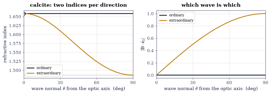
Fig. 326 The two refractive indices of calcite as the wave normal turns away from the optic axis. Left: the ordinary index (dark) sits at \(n_o = 1.6584\) for every direction, a flat line to fourteen decimal places, while the extraordinary index (amber) falls along the ellipse of eq-co-uniaxial from \(n_o\) on the axis to \(n_e = 1.4864\) at right angles to it; the dotted lines mark those two values and the open circle marks the single direction, \(\theta = 0\), at which the two waves are indistinguishable. Right: the component of each wave’s displacement along the optic axis, \(|\mathbf D\cdot\hat{\mathbf e}_3|\), which is the labelling made visible: it is identically zero for the ordinary wave at every direction and rises as \(\sin\theta\) for the extraordinary one, except at \(\theta = 0\) itself where the two indices coincide and the polarizations are not defined.#
Exercise 4 — Walk-off: the ray goes where the wave normal does not (student)#
This is the exercise §3.16 was written for. Exercise 4 of that notebook measured the angle between \(\mathbf D\) and \(\mathbf E\) over the whole sphere of field directions, found it vanishing on the three principal axes and reaching a maximum in between, and left it as a statement about vectors. Here it becomes a statement about where light goes.
The argument is the one sketched in the theory and worth repeating slowly, because everything hangs on it (Fig. 327). The wavefronts of a plane wave are the surfaces of constant phase, and they advance along \(\hat{\mathbf s}\); the displacement \(\mathbf D\) lies in those wavefronts because \(\nabla\cdot\mathbf D=0\). The energy, however, flows along \(\mathbf S=\mathbf E\times\mathbf H\), which is perpendicular to \(\mathbf E\), not to \(\mathbf D\). Since \(\mathbf H\) is perpendicular to all four vectors, the pair \((\mathbf E,\mathbf S)\) is the pair \((\mathbf D, \hat{\mathbf s})\) turned rigidly through one angle, so the angle between the ray and its own wave normal is the angle between \(\mathbf E\) and \(\mathbf D\). A beam therefore leaves its own wavefront behind, drifting sideways as it goes, and the beam that emerges from a crystal is displaced from the one that would have emerged had the crystal been glass. The name for the angle is walk-off, and for a uniaxial crystal it is Eq. 305, largest at Eq. 306.
It is worth noticing before computing anything that Eq. 306 and the maximum \(\mathbf D\)–\(\mathbf E\) angle of §3.16 are the same formula written in different letters, \(\tan\alpha_{\max}=(\varepsilon_3-\varepsilon_1)/2\sqrt{\varepsilon_1 \varepsilon_3}\) becoming \(\tan\rho_{\max}=(n_o^2-n_e^2)/2n_on_e\) under \(\varepsilon_i=n_i^2\). The number that notebook obtained by turning a calcite crystal on a turntable in a static field, \(6.26^\circ\), is about to reappear as an angle in an optics laboratory.
Part a) Write ray_direction(eps, s_hat, D_hat) returning the unit Poynting
direction from Eq. 304. Recover the field as
numpy.linalg.solve(eps, D_hat), form \(\mathbf H\propto\hat{\mathbf s}\times\mathbf E\)
and then \(\mathbf S=\mathbf E\times\mathbf H\) with two calls to numpy.cross, and
normalize with numpy.linalg.norm.
Write this one yourself — the implementation is the lesson.
Part b) Using the sweep of Exercise 3 over 2001 angles on \([0,\pi/2]\) and the
extraordinary polarizations collected there, compute the walk-off angle at each
direction as \(\arccos(\hat{\mathbf S}\cdot\hat{\mathbf s})\), guarding the cosine with
numpy.clip(..., -1.0, 1.0) first for the reason
§3.16 gives: the true angle vanishes at both ends of
the sweep and rounding can push the cosine one ulp past one, where arccos returns
nan. Compare the whole curve with Eq. 305 and report the two endpoint
values.
Part c) Locate the maximum with scipy.optimize.minimize_scalar applied to
\(-\rho(\theta)\) with method="bounded", bounds=(0.02, numpy.pi/2 - 0.02) and
options={"xatol": 1e-12} — a bracketed one-dimensional minimizer, because the wanted
quantity is the location of a smooth interior maximum and a grid search resolves it only
to the grid spacing. Compare both the maximum and its position with
Eq. 306.
Part d) Close the loop with §3.16. For each direction in the sweep
form the extraordinary field \(\mathbf E\) and pass it to the angle_DE of the Setup,
which §3.16 built; report the largest difference
between that angle and the walk-off angle of Part b over the whole sweep.
Part e) Put a number on the double image. A calcite plate of thickness \(d=10.00\,\)mm is cut so that its optic axis makes the angle \(\theta^\star\) of Eq. 306 with the face normal, and unpolarized light arrives at normal incidence. Both wave normals then go straight through, so the ordinary ray does too, while the extraordinary ray leaves the far face displaced sideways by \(d\tan\rho_{\max}\). Report that displacement in millimetres.
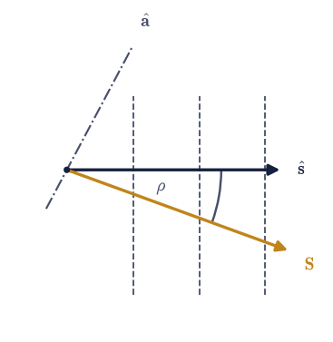
Fig. 327 Walk-off in a uniaxial crystal, drawn in the plane containing the wave normal and the optic axis. The dashed lines are successive wavefronts, surfaces of constant phase which advance along the wave normal \(\hat{\mathbf s}\) at speed \(c/n\); the dash-dotted line is the optic axis \(\hat{\mathbf a}\). Energy travels instead along the ray \(\mathbf S\), at the walk-off angle \(\rho\) to \(\hat{\mathbf s}\), so the beam slides along its own wavefronts as it propagates and emerges from the far face displaced sideways. The angle is drawn at \(20^\circ\) for legibility; in calcite its largest value is \(6.26^\circ\), which over a centimetre of crystal is about a millimetre of displacement.#
walk-off vs eq-co-walkoff: max|Δ| = 2.69e-13
endpoints: ρ(0°) = 0.00e+00°, ρ(90°) = 0.00e+00°
measured  ρ_max = 6.2611709° at θ* = 41.869415°
eq-co-walkoffmax: ρ_max = 6.2611709° at θ* = 41.869415°
walk-off vs the D–E angle of §3.16: max|Δ| = 7.19e-13
a 10.00 mm calcite plate cut at θ* displaces the e-ray by 1.0972 mm
Validation 4#
The first two checks grade the computation against Eq. 305 and
Eq. 306, neither of which entered it: the walk-off came out of a Poynting
vector built from an eigenvector, and the closed forms came out of algebra. The third is
a physical statement with teeth, since a mislabelled mode or a wrong cross product would
not vanish at both ends: reverse either cross product in Eq. 304 and the
angle comes back as \(180^\circ\) rather than zero. It reads as an exact zero rather than a
round-off one because at both ends the displacement lands on a principal direction, where
the field is parallel to it and there is no arithmetic left to lose. The fourth is the connection to
§3.16, and it deserves an honest word about what it
tests: that the ray angle equals the \(\mathbf D\)–\(\mathbf E\) angle is a theorem given
Eq. 299, so this check does not add independent physics. What it does test is
that the pair \((n,\mathbf D)\) the engine returned genuinely satisfies that equation, by a
route entirely different from Exercise 1’s residual: if the eigenproblem had been solved
in the wrong plane, the two angles would part company immediately. Its tolerance is set by
arithmetic rather than by physics: both angles are an arccos of a cosine within
\(10^{-6}\) of one wherever the walk-off is small, and arccos is ill-conditioned there,
with an error growing like \(1/\rho\), so a floor near \(10^{-12}\) is the best the comparison
can do at the ends of the sweep.
✓  the computed walk-off matches eq-co-walkoff at every one of 2001 directions   [max|Δ| = 2.68981e-13 (rtol=0, atol=1e-10)]
✓  the largest walk-off is 6.2611709° at θ* = 41.869414°, as eq-co-walkoffmax predicts   [max|Δ| = 4.87089e-10 (rtol=1e-06, atol=1e-09)]
✓  the ray follows its wave normal exactly along the optic axis and exactly across it   [max|Δ| = 0 (rtol=0, atol=1e-14)]
✓  the ray–normal angle IS the D–E angle of §3.16, at every direction   [max|Δ| = 7.1875e-13 (rtol=0, atol=1e-12)]
True
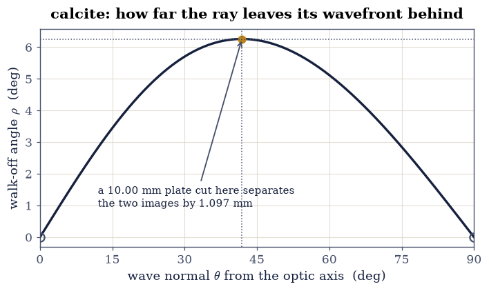
Fig. 328 The walk-off angle of the extraordinary wave in calcite against the direction of its wave normal, measured from the optic axis. The curve is computed from the Poynting vector of the solved mode; the dotted lines and the amber point mark the maximum \(\rho_{\max} = 6.2612^\circ\) at \(\theta^\star = 41.869^\circ\), which is the closed form eq-co-walkoffmax and not a fit. The angle vanishes at both ends, where the wave normal lies along a principal direction and the displacement and the field are parallel, and the open circles mark those two zeros. The annotation converts the peak into the sideways displacement of the ray after \(10.00\) mm of crystal, \(1.097\) mm, which is the separation between the two images seen through a calcite rhomb.#
Exercise 5 — Double refraction at a calcite surface (student)#
So far the wave was already inside the crystal. Getting it in is where the word birefringence comes from, and it needs one result from §3.15 and nothing else. That notebook showed that Snell’s law is not an independent postulate but phase matching: a boundary condition has to hold at every point of the surface at once, which forces every wave present to share the same tangential wavevector, and with \(k=n\omega/c\) that is \(n_1\sin\theta_i=n_2\sin\theta_t\). Nothing in that argument assumed one refracted wave. In a crystal there are two, so the condition has to be satisfied twice, once for each index (Fig. 329).
The ordinary branch is easy, because its index is the constant \(n_o\) of Exercise 3, so plain Snell applies unchanged. The extraordinary branch is not, because its index depends on the very angle we are solving for: the refracted wave normal makes some angle with the optic axis, and that angle sets the index, which sets the refraction angle. What is a formula for the ordinary ray becomes a transcendental equation for the extraordinary one,
with \(n^{(e)}(\theta_t)\) evaluated by the engine of Exercise 1. Then the two rays part company a second time, because the extraordinary ray walks off from its own wave normal by the angle of Exercise 4 while the ordinary one does not.
The geometry: light in air, \(n_1=1\), arrives at a flat calcite face at \(\theta_i=30.00^\circ\) from the surface normal. Take the laboratory frame with \(\hat{\mathbf e}_3\) along the inward surface normal and \(\hat{\mathbf e}_1\) in the surface, both in the plane of incidence. The crystal is cut so that its optic axis lies in the plane of incidence at \(\gamma=45.00^\circ\) from the inward normal.
Part a) Build the laboratory-frame permittivity. Take
\(\mathsf R_c=\) rotation_matrix((0, 1, 0), numpy.deg2rad(45)) from the Setup, which
carries \(\hat{\mathbf e}_3\) onto \((\sin\gamma,0,\cos\gamma)\), and apply
transform_tensor(EPS_CALCITE, R_c). The optic axis in the laboratory is then the third
column R_c[:, 2]. Print the tensor: it is no longer diagonal, which is why the
polynomial route of Exercise 2 is unavailable here and the eigenproblem is not.
Part b) The ordinary branch. Compute
\(\theta_o=\arcsin(\sin\theta_i/n_o)\) with numpy.arcsin, then evaluate
wave_normal_modes on the laboratory tensor at that direction and read back the index
of the mode whose \(\mathbf D\) is perpendicular to the laboratory optic axis
(numpy.argmin on \(|\mathbf D\cdot\hat{\mathbf a}|\), as in Exercise 3). It must return
\(n_o\) to machine precision, which is the statement that plain Snell was legitimate.
Part c) The extraordinary branch. Solve Eq. 312 with
scipy.optimize.brentq on the bracket \([1^\circ,60^\circ]\) in radians and
xtol=1e-14, the residual function evaluating the extraordinary index at each trial
angle through wave_normal_modes. A bracketing method is the right one here: the
residual is continuous and changes sign across the bracket, and no derivative is
available in closed form. Report the refracted wave-normal angle and its index.
Part d) The rays. For each branch feed the solved wave normal and its polarization
to the ray_direction built in Exercise 4, and report the angle each ray makes with
the surface normal, via numpy.arctan2(S[0], S[2]). Report the two splittings: between
the wave normals, and between the rays. Check the extraordinary walk-off against
Eq. 305 evaluated at the angle between its wave normal and the optic axis.
Part e) State what a viewer sees. Two rays leave the entry point in two different directions, so a mark viewed through the crystal appears twice, and the two images are oppositely polarized.
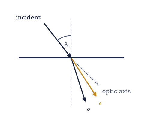
Fig. 329 Double refraction at a calcite surface, with light arriving from air at \(\theta_i\) to the inward surface normal (dotted). The crystal fills the lower half plane and its optic axis (dash-dotted, drawn inside the crystal only) lies in the plane of incidence. Phase matching admits two refracted waves rather than one: the ordinary wave, whose index is the constant \(n_o\) so that plain Snell holds for it, and the extraordinary wave, whose index depends on the very angle being solved for. Their rays separate further still, because the extraordinary ray walks off from its own wave normal by the angle \(\rho\) while the ordinary ray does not. The three angles are drawn far apart for legibility; the computed values are \(17.547^\circ\) and \(12.614^\circ\) for the two rays, from wave normals only \(0.452^\circ\) apart.#
calcite in the laboratory frame (no longer diagonal):
[[ 2.479838  0.       -0.270453]
 [ 0.        2.750291  0.      ]
 [-0.270453  0.        2.479838]]
optic axis in the laboratory: [0.707107 0.       0.707107]
ordinary wave normal: 17.547444°, index returned 1.658400000000
extraordinary wave normal: 17.999502°, index 1.618077282
   phase-matching residual at the root: 5.6e-17
ordinary ray at 17.547444°, extraordinary ray at 12.613778°
e-wave normal sits 27.0005° from the optic axis
   its walk-off: 5.385723° (eq-co-walkoff: 5.385723°)
wave normals split by 0.452058°; rays split by 4.933665°
Validation 5#
The residual of Eq. 312 at the root is not validated below, because
brentq drove it to zero by construction and a check on it would report the solver’s
convergence rather than any physics; it is printed above for that reason and no other.
What is checked is independent of it. The ordinary index comes back as \(n_o\) from a
tensor that is not diagonal, in a frame the closed form knows nothing about. The
extraordinary index at the solved angle matches Eq. 303 evaluated at the
angle between that wave normal and the optic axis, which is a comparison between a
laboratory-frame eigenproblem and a crystal-frame formula. Its walk-off matches
Eq. 305 at the same angle. And the last check is the physics a viewer sees:
most of the separation between the two images is made by walk-off, not by the difference
in refraction angle.
✓  the ordinary index is n_o even in a tilted laboratory frame, so plain Snell was exact for it   [got 1.6584 vs expected 1.6584 (rtol=0, atol=1e-13)]
✓  the extraordinary index at its refracted angle matches eq-co-uniaxial at 27.00° from the axis   [got 1.61808 vs expected 1.61808 (rtol=1e-12, atol=1e-09)]
✓  and its ray walks off from its own wave normal by the 5.386° that eq-co-walkoff predicts   [got 0.0939986 vs expected 0.0939986 (rtol=1e-09, atol=1e-09)]
✓  the doubled image is made mostly by walk-off, not by the split in refraction angle   [rays 4.9337° apart vs wave normals 0.4521°]
True
Exercise 6 — The index surface and the wave surface (student)#
The engine returns two numbers per direction, and a function of direction is best looked at as a surface. Plot the index as a radius, \(\mathbf r=n(\hat{\mathbf s})\, \hat{\mathbf s}\), and the result is the index surface, with two sheets because there are two indices. Everything the last four exercises established is a statement about its shape: the ordinary sheet is a sphere because \(n_o\) does not depend on direction, the extraordinary sheet is a spheroid because \(n^{(e)}\) traces the ellipse of Eq. 303, and the two meet only where those agree, which by Eq. 303 is the optic axis and nowhere else. A uniaxial crystal has exactly one direction along which light does not split, which is what gives the class its name.
The same information carried by rays rather than wave normals is the wave surface, and it is the older object: it is Huygens’ secondary wavelet, the locus reached in unit time by energy leaving a point inside the crystal, drawn in the Traité de la Lumière of 1690 as a sphere and a spheroid nested together, more than a century before anyone could say what light was. Building it needs both pieces of Exercise 4, since a ray leaves along \(\hat{\mathbf S}\) rather than \(\hat{\mathbf s}\) and covers the hypotenuse of the walk-off triangle, so its speed is
The two surfaces are not the same shape. The extraordinary sheet of the index surface is Eq. 307, with semi-axis \(n_o\) along the optic axis and \(n_e\) across it; the extraordinary sheet of the wave surface is Eq. 308, with semi-axis \(c/n_o\) along the axis and \(c/n_e\) across it. Both are worth having, and neither is the index ellipsoid of §3.16, whose semi-axes are \(n_o\) across the optic axis and \(n_e\) along it. Three ellipsoids, three jobs, and keeping them apart is most of the difficulty a first pass at crystal optics has.
Part a) Build the index-surface meridian. Sweep \(\theta\) over 721 angles spaced
linearly on \([0,2\pi]\) with numpy.linspace, evaluate the wave_normal_modes and
wave_normal of Exercise 1 on calcite at each, label the modes as in Exercise 3, and
form the two point sets \(n\,\hat{\mathbf s}\) with a broadcast multiply. Report
numpy.ptp of the ordinary radius from numpy.linalg.norm, and the largest deviation
of the extraordinary points from Eq. 307, evaluating
\(x^2/n_e^2+z^2/n_o^2\) and comparing with \(1\).
Part b) Build the wave-surface meridian. At each direction take the extraordinary
ray from the ray_direction of Exercise 4, its walk-off angle, and the ray speed
Eq. 313, and form the point \(v_{\rm ray}\hat{\mathbf S}\). Check it against
Eq. 308 the same way. Report the two extreme ray speeds in m/s, and note
that the ordinary sheet is a sphere of radius \(c/n_o\).
Part c) Measure the contact. Evaluate the gap between the two indices,
\(n_o-n^{(e)}(\theta)\), from the closed form Eq. 303 written as a vectorized
numpy expression on the explicit array \(\theta=[10^{-3},2\times10^{-3},4\times10^{-3},
8\times10^{-3}]\) radians, and report the ratios between successive values with a
shifted-slice division. A gap growing by a factor four
per doubling of \(\theta\) means the sheets touch quadratically rather than crossing; fit
the exponent with numpy.polyfit of degree 1 on \(\ln(\text{gap})\) against
\(\ln\theta\) and report the slope. Confirm the gap is strictly positive at every
\(\theta>0\) in the sweep of Exercise 3, so the touching happens at the optic axis alone.
Part d) Plot both meridians side by side, with the optic axis vertical, on axes with equal aspect ratio so the shapes are not distorted, and put an inset on the index-surface panel magnifying the neighbourhood of the axis so the tangential contact is visible (Fig. 330).
ordinary sheet radius: 1.6584000000, ptp 4.44e-16
extraordinary sheet vs eq-co-indexsurface: max|Δ| = 6.66e-16
extraordinary sheet vs eq-co-raysurface: max|Δ| = 8.88e-16
extraordinary ray speed runs 1.8077e+08 to 2.0169e+08 m/s
ordinary sheet is a sphere of radius c/n_o = 1.8077e+08 m/s
gap at θ = [0.001 0.002 0.004 0.008]: [2.030e-07 8.120e-07 3.248e-06 1.299e-05]
ratios between successive gaps: [3.99999 3.99998 3.9999 ]
fitted contact exponent: 1.999985
smallest index gap anywhere off the optic axis: 1.252e-07
Validation 6#
The first two checks identify the shapes, and they are not the same check twice. The index-surface one re-expresses the closed form of Exercise 3 in Cartesian coordinates, so what it adds is the identification of the semi-axes rather than new physics. The wave-surface one is genuinely new information: its points came from the Poynting direction and the ray speed Eq. 313, neither of which appears in Eq. 308, and landing on that ellipsoid to machine precision is the statement that Huygens’ spheroid is the right one. The contact exponent turns “the sheets touch” into a measurement, and the last check says the touching happens nowhere else.
✓  the index surface is a sphere of radius n_o and the spheroid eq-co-indexsurface   [sphere ptp 4.4e-16, spheroid residual 6.7e-16]
✓  the ray points built from the Poynting vector lie on Huygens' spheroid eq-co-raysurface   [got 8.88178e-16 vs expected 0 (rtol=0, atol=1e-13)]
✓  the two sheets touch the optic axis quadratically: the gap grows fourfold per doubling of θ   [got 1.99999 vs expected 2 (rtol=0.003, atol=1e-09)]
✓  and they touch there alone: every other direction splits light into two waves   [smallest gap off the axis = 1.25e-07]
True
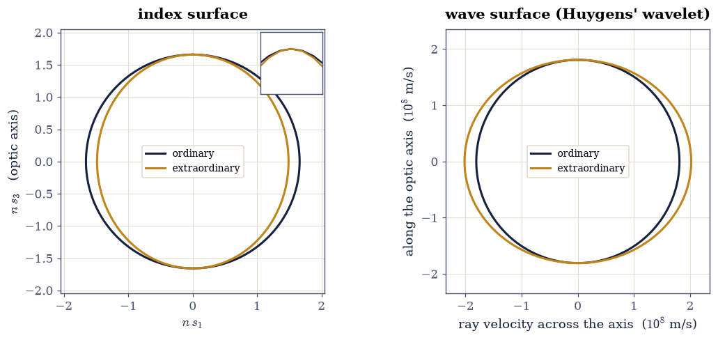
Fig. 330 The two surfaces of calcite, drawn as meridian sections in the plane containing the optic axis, which is vertical in both panels; each full surface is generated by revolving its section about that axis. Left: the index surface, the refractive index plotted as a radius. The ordinary sheet (dark) is a circle of radius \(n_o = 1.6584\) and the extraordinary sheet (amber) is the ellipse eq-co-indexsurface with semi-axis \(n_o\) along the optic axis and \(n_e = 1.4864\) across it, so the extraordinary sheet lies inside the ordinary one everywhere except on the axis; the inset magnifies the top of the axis by a factor of about forty, where the two sheets meet tangentially rather than crossing. Right: the wave surface, the distance travelled by energy in unit time, which is Huygens’ construction of 1690. Here the ordinary sheet is the circle of radius \(c/n_o\) and the extraordinary sheet is the ellipse eq-co-raysurface with the semi-axes exchanged, so for this negative crystal the extraordinary wavelet lies outside the ordinary one. Both panels use equal aspect ratios.#
Exercise 7 — Wave plates, from the phase difference (student)#
Everything so far has been about the two waves separately. What a wave plate does is put them back together and let them interfere (Fig. 331).
Cut a slab so that the optic axis lies in the entrance face, and send light in along the face normal. The wave normal is then perpendicular to the optic axis, and Exercise 3 says the two allowed polarizations have indices exactly \(n_o\) and \(n_e\), with \(\mathbf D\) perpendicular to the axis and along it. There is a second reason to cut a plate this way, and it is the one Exercise 4 supplies: at \(\theta=90^\circ\) the walk-off vanishes for both waves, so the two beams stay on top of each other instead of separating inside the plate. The plate is then a pure phase device. The faster polarization (the one with the smaller index) is called the plate’s fast axis, and after a thickness \(d\) the two have accumulated the phase difference Eq. 309. Choosing \(d\) to make \(\Delta\phi=\pi/2\) gives a quarter-wave plate and \(\Delta\phi=\pi\) a half-wave plate.
What that does to the light is a question about the real electric field, and it does not need any new formalism to answer. Linearly polarized light entering at azimuth \(\psi\) to the plate’s axes leaves as
whose tip traces a closed curve once per optical cycle. That curve is an ellipse, and
rather than assert what kind we trace it and measure it. Two measurements suffice: the
time-averaged second-moment matrix \(M_{ab}=\langle E_aE_b\rangle\), whose eigenvalues are
half the squared semi-axes and whose eigenvectors give the ellipse’s orientation, and the
signed area the curve encloses, whose sign is the handedness of the rotation. The
eigenvalue step is numpy.linalg.eigh on a \(2\times2\) real symmetric matrix, which is
the same tool as the engine of Exercise 1 doing an entirely different job.
Part a) Confirm the cut. Evaluate the wave_normal_modes of Exercise 1 on calcite
at \(\hat{\mathbf s}=(1,0,0)\), perpendicular to the optic axis, and check that the two
indices are exactly \(n_o\) and \(n_e\) and the two polarizations are \(\hat{\mathbf e}_2\) and
\(\hat{\mathbf e}_3\). Then feed both to the ray_direction of Exercise 4 and report the
walk-off angle of each.
Part b) Compute plate thicknesses from Eq. 309 at \(\lambda=589.3\,\)nm, for calcite (\(\Delta n=0.1720\)) and for quartz (\(n_o=1.54424\), \(n_e=1.55335\), so \(\Delta n=0.00911\)): the quarter-wave and half-wave thickness of each, and the multi-order quarter-wave thickness \(d_m=(m+\tfrac14)\lambda/\Delta n\) for \(m=10\). Comment on which of the four is a slab a person could handle.
Part c) Write polarization_trace(psi, delta, n_samples=20000) returning the two
field components of Eq. 314 sampled over one optical cycle, using
numpy.linspace(0, 2*numpy.pi, n_samples, endpoint=False) for the phase — the open
endpoint matters, since a duplicated first point biases both the average and the enclosed
area. Write ellipse_parameters(Ex, Ey) returning the semi-major axis \(A\), the semi-minor
axis \(B\), the azimuth of the major axis folded into \((-90^\circ,90^\circ]\), and the
signed area. Build \(M\) with numpy.mean on the three products, diagonalize with
numpy.linalg.eigh, take \(A,B=\sqrt{2\lambda_\pm}\) after clipping the eigenvalues at zero
with numpy.clip (a perfectly linear state gives a numerically tiny negative one), read
the azimuth from the major eigenvector with numpy.arctan2, and get the signed area from
the shoelace formula \(\tfrac12\sum(x_i y_{i+1}-x_{i+1}y_i)\) using numpy.roll.
Part d) The quarter-wave plate at \(\psi=45^\circ\). Report \(B/A\), which must be \(1\):
linear light in, circular light out. Report the signed area that ellipse_parameters returns for \(\Delta\phi=+\pi/2\) and
for \(\Delta\phi=-\pi/2\), which are the two circular handednesses, and check that the
magnitude of the area agrees with \(\pi AB\) from the second-moment axes. Do not check the
azimuth: a circle has no major axis, and whatever eigh returns for it is arbitrary.
Part e) The half-wave plate. For \(\psi=10^\circ,20^\circ,\ldots,80^\circ\) report the output azimuth and \(B/A\). The output stays linear and its azimuth comes out at \(-\psi\), which is the input reflected in the plate’s fast axis: a half-wave plate rotates a linear polarization by twice the angle between it and the axis.
Part f) Then the quarter-wave plate at general \(\psi\), against Eq. 310: report \(\sin2\chi\) from the measured \(\tan\chi=B/A\) beside \(\sin2\psi\).
Part g) Why the thick plate is the fragile one. The retardance Eq. 309 is inversely proportional to \(\lambda\), so a plate cut for \(589.3\,\)nm is wrong at \(632.8\,\)nm by \(\Delta\phi_0(\lambda_0/\lambda-1)\), where \(\Delta\phi_0\) is its total design retardance. Compute that error for the zero-order quartz quarter-wave plate (\(\Delta\phi_0=\pi/2\)) and for the \(m=10\) plate (\(\Delta\phi_0=2\pi\times10.25\)), and report their ratio. Hold \(\Delta n\) fixed at its sodium-D value while doing so, and say plainly that this isolates the geometric part only: a real plate also has \(\Delta n(\lambda)\), which is the dispersion §3.15 built and this notebook switched off.
Part h) Animate the state changing with depth. Ramp \(\Delta\phi\) from \(0\) to \(\pi\) over 121 frames at \(\psi=45^\circ\), which is a beam advancing through a half-wave plate, drawing at each depth the traced curve and the instantaneous field vector (Fig. 332). Record \(B\) at each frame; it must follow \(B(\Delta\phi)=\sqrt{(1-|\cos\Delta\phi|)/2}\), rising from zero to \(A\) at the quarter-wave depth and falling back to zero at the half-wave depth.
With your assistant
Part h is plumbing: a FuncAnimation, a line artist for the traced curve, a second one
for the instantaneous field vector, equal aspect ratios, a running title. Ask your
assistant to write it, then run the check that decides whether the picture is telling the
truth: take the frame at which \(\Delta\phi=\pi/2\), feed its own traced \((E_x,E_y)\) back
through ellipse_parameters, and confirm \(B/A=1\) there and \(B/A=0\) at the last frame. If
those two numbers are not \(1\) and \(0\), the animation is showing something other than a
quarter-wave and a half-wave plate, however smoothly it plays. The check is yours.
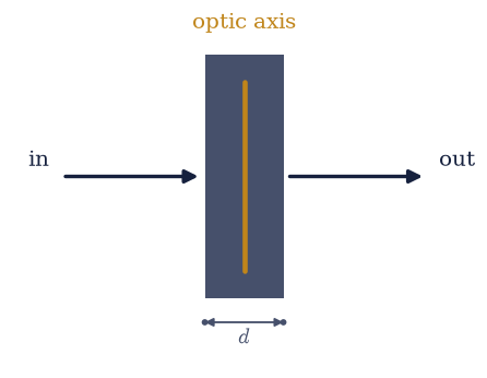
Fig. 331 A wave plate, cut so that the optic axis (amber) lies in the entrance face rather than along the beam. Light enters from the left travelling along the face normal, so the wave normal is perpendicular to the optic axis; the two allowed polarizations are then exactly ordinary and extraordinary, with indices \(n_o\) and \(n_e\), and both have zero walk-off, so the two beams stay superposed inside the slab instead of separating. Over the thickness \(d\) they accumulate the phase difference \(\Delta\phi = 2\pi|n_o - n_e|d/\lambda\) of eq-co-retardance, and it is that leftover phase, not any change of direction, that the plate exists to produce.#
indices across the optic axis: [1.6584 1.4864]
their polarizations (rows):
[[0. 1. 0.]
 [0. 0. 1.]]
walk-off of each: [0. 0.] deg
calcite Δn = 0.1720:  λ/4 plate    856.5 nm, λ/2 plate   1713.1 nm
quartz  Δn = 0.00911: λ/4 plate    16.17 µm, λ/2 plate    32.34 µm
quartz multi-order (m = 10) λ/4 plate: 663.0 µm
λ/4 at ψ = 45°: A = 0.707106781187, B = 0.707106781187, B/A = 1.000000000000
   signed area +1.57079630 for δ = +π/2 and -1.57079630 for δ = −π/2
   πAB from the second moments: 1.57079633
half-wave plate:  ψ (deg) → output azimuth (deg), B/A
    10.0 → -10.000000, 1.86e-09
    20.0 → -20.000000, 0.00e+00
    30.0 → -30.000000, 5.27e-09
    40.0 → -40.000000, 5.27e-09
    50.0 → -50.000000, 0.00e+00
    60.0 → -60.000000, 0.00e+00
    70.0 → -70.000000, 0.00e+00
    80.0 → -80.000000, 0.00e+00
quarter-wave plate:  sin 2χ measured vs sin 2ψ
   ψ =  10.0°: 0.3420201433 vs 0.3420201433
   ψ =  20.0°: 0.6427876097 vs 0.6427876097
   ψ =  30.0°: 0.8660254038 vs 0.8660254038
   ψ =  40.0°: 0.9848077530 vs 0.9848077530
   ψ =  50.0°: 0.9848077530 vs 0.9848077530
   ψ =  60.0°: 0.8660254038 vs 0.8660254038
   ψ =  70.0°: 0.6427876097 vs 0.6427876097
   ψ =  80.0°: 0.3420201433 vs 0.3420201433
at 632.8 nm the zero-order quartz λ/4 plate is off by 0.10798 rad
the m = 10 plate is off by 4.42717 rad
ratio 41.0000 (Δn held at its sodium-D value)
animated minor axis vs its closed form: max|Δ| = 2.12e-15
Validation 7#
The first check is about the cut rather than the plate: a wave normal perpendicular to the optic axis has both its walk-off angles vanish, which is why a plate made this way keeps its two beams superposed. That one is an exact zero for the reason Exercise 4 gave, both displacements landing on principal axes; what it can still catch is a wrong Poynting construction or a plate cut the other way, either of which returns something far from it. Then the states themselves, each measured from a traced curve rather than asserted: circular light out of a quarter-wave plate at \(45^\circ\), a linear state rotated to \(-\psi\) by a half-wave plate at every one of eight input azimuths, and the ellipticity of Eq. 310, which the trace never used. The shoelace area against \(\pi AB\) is a cross-check between two independent measurements of the same ellipse, a polygon integral and a covariance eigenproblem. The retardance-error ratio is exactly \((m+\tfrac14)/\tfrac14=41\) and is the reason zero-order plates exist. The animation’s validation, as the course requires, tests the animated data: the minor axis recovered from each frame’s own trace against its closed form.
✓  a wave normal across the optic axis has zero walk-off in both modes: the plate cut is clean   [largest walk-off 0.0e+00 deg]
✓  and its two indices are exactly n_o and n_e, so eq-co-retardance uses the measured Δn   [max|Δ| = 2.22045e-16 (rtol=0, atol=1e-14)]
✓  a quarter-wave plate at 45° makes circular light, of either handedness as δ changes sign   [B/A = 1.0000000000, areas +1.5708 and -1.5708]
✓  the area the traced curve encloses agrees with πAB from the second-moment axes   [got 1.5708 vs expected 1.5708 (rtol=1e-06, atol=1e-09)]
✓  a half-wave plate reflects a linear polarization in its own axis, taking ψ to −ψ   [max|Δ| = 7.77156e-16 (rtol=0, atol=1e-09)]
✓  and leaves it linear: the minor axis stays at zero for every input azimuth   [largest B/A over the eight inputs = 5.3e-09]
✓  the quarter-wave ellipticity follows sin 2χ = sin 2ψ sin δ of eq-co-ellipticity   [max|Δ| = 1.11022e-16 (rtol=1e-09, atol=1e-09)]
✓  the m = 10 plate is 41 times more wavelength-sensitive than the zero-order one   [got 41 vs expected 41 (rtol=1e-09, atol=1e-09)]
✓  the animated state follows B(δ) = √[(1 − |cos δ|)/2] at every depth in the plate   [max|Δ| = 2.12157e-15 (rtol=0, atol=1e-12)]
True
Fig. 332 Animation of a linear polarization at \(45^\circ\) to the plate axes as it advances through a half-wave plate. The frame index is the depth, which enters only through the accumulated retardance \(\Delta\phi\) of eq-co-retardance, printed above the panel in units of \(\pi\); the amber curve is the closed path the tip of the electric vector traces over one optical cycle at that depth, and the dark arrow is the instantaneous field, which continues to rotate as the depth advances. The state opens linear, opens out into an ellipse, becomes exactly circular at the quarter-wave depth, closes again, and arrives at the far face linear once more but reflected in the plate axis, at \(-45^\circ\). The dotted diagonals mark the input azimuth and its reflection.#
Exercise 8 — Two optic axes, and where this notebook stops (student)#
Everything since Exercise 3 has been uniaxial, and the engine of Exercise 1 never was. It takes a symmetric tensor and a direction and returns two indices, and it does not know or care whether two of the principal values happen to coincide. So the biaxial case costs no new code at all, and it is worth spending one exercise to see what the same machine says about it, and to be explicit about what this notebook then declines to do.
The geometry is the one §3.16 built. The two indices for a direction are the semi-axes of the central section of the index ellipsoid perpendicular to \(\hat{\mathbf s}\), so light fails to split exactly when that section is a circle. For a spheroid that happens once; for a general ellipsoid with \(n_1<n_2<n_3\) it happens twice, and finding where takes three lines. Any section contains at least one of the ellipsoid’s own axes when \(\hat{\mathbf s}\) lies in a principal plane, so look in the \(\hat{\mathbf e}_1\)–\(\hat{\mathbf e}_3\) plane and write \(\hat{\mathbf s}=(\sin\beta,0,\cos\beta)\). The section perpendicular to it is spanned by \(\hat{\mathbf e}_2\), of radius \(n_2\), and by \((\cos\beta,0,-\sin\beta)\), whose radius \(r\) on the indicatrix obeys \(1/r^2=\cos^2\beta/n_1^2+\sin^2\beta/n_3^2\). Setting \(r=n_2\) gives Eq. 311, with two solutions \(\pm\beta\) straddling the \(\hat{\mathbf e}_3\) axis. Two optic axes: hence biaxial, and hence the name of the uniaxial class, which has one.
The specimen is the model crystal of §3.16, \(\boldsymbol\varepsilon=\mathrm{diag}(2.40,\,3.00,\,4.20)\), whose principal indices are \(n_1=1.549193\), \(n_2=1.732051\) and \(n_3=2.049390\).
Part a) Map the splitting over the sphere. Build 91 polar angles on \([0,\pi]\) and
181 azimuths on \([0,2\pi]\) with numpy.linspace and numpy.meshgrid(..., indexing="ij"),
form the unit vectors \((\sin\vartheta\cos\varphi,\sin\vartheta\sin\varphi,
\cos\vartheta)\), and evaluate \(|n_1-n_2|\) from the wave_normal_modes of Exercise 1 at
each. Report the smallest and largest splitting, and the direction at which the smallest
occurs; there are four such directions on the full sphere, being two axes and their
antipodes (Fig. 333). The map’s minimum will not be zero, and that is the
grid rather than the physics: with a \(2^\circ\) spacing no sample sits exactly on an axis,
so measure instead the angle between the location of the minimum and the nearest
direction \((\pm\sin\beta,0,\pm\cos\beta)\) that Eq. 311 predicts, with
numpy.arccos on the dot products. That angle is what the map can honestly be said to
resolve; Part b then locates the axis properly.
Part b) Locate one axis precisely. In the \(\hat{\mathbf e}_1\)–\(\hat{\mathbf e}_3\)
plane the two modes can be told apart the way Exercise 3 told them apart: one has
\(\mathbf D\) along \(\hat{\mathbf e}_2\) and the other has it in the plane. Form the
signed difference, the in-plane index minus the \(\hat{\mathbf e}_2\) one, which changes
sign at the axis where \(|n_1-n_2|\) merely touches zero, and solve it with
scipy.optimize.brentq on the bracket \([1^\circ,89^\circ]\) in radians with xtol=1e-14
— a bracketing method again, since the residual is continuous and changes sign, and the
unsigned gap would defeat any root-finder.
Part c) Compare with Eq. 311, evaluating it as
numpy.arctan2(numpy.sqrt(u1 - u2), numpy.sqrt(u2 - u3)) with \(u_i=1/\varepsilon_i\), a
form that stays finite when the second difference vanishes. Report the two indices at the
axis, which must both be \(n_2=\sqrt{3}=1.7320508\): the circular section has the
intermediate radius, and it is the intermediate index that an optic axis carries.
Part d) Check the uniaxial limits with the same two routes. Setting
\(\varepsilon_2=\varepsilon_1=2.40\) makes the crystal uniaxial about \(\hat{\mathbf e}_3\)
and Eq. 311 gives \(\beta=0\); setting \(\varepsilon_2=\varepsilon_3=4.20\)
makes it uniaxial about \(\hat{\mathbf e}_1\) and gives \(\beta=90^\circ\). Confirm both with
the engine: call wave_normal_modes on each tensor at \(\beta=0\) and at \(\beta=90^\circ\)
and take numpy.diff of the returned pair. One splitting is zero and the other is not. The uniaxial crystals are the two ends of the biaxial
family, with the two optic axes merged into one.
Part e) Say what has not been done. This notebook gives the biaxial case its optic axes and stops there. It does not build the biaxial walk-off, the four-sheeted meridian section of the wave surface, or conical refraction — Hamilton’s 1832 prediction, and Lloyd’s observation two months later, that a narrow beam sent exactly along an optic axis of a biaxial crystal emerges as a hollow cone. The reason is honesty about conventions rather than difficulty: the sign of \(\beta\), which axis it is measured from, and whether a crystal is called positive or negative all differ between standard sources, and a treatment that quietly mixes two of them produces figures that are wrong in a way no validation catches. Born and Wolf [BW99] (§15.3) develop the biaxial case in full and state their conventions explicitly, which is what a serious treatment requires.
principal indices: [1.549193 1.732051 2.04939 ]
smallest splitting on the sampled sphere: 7.416e-03
largest splitting: 0.500197
the minimum sits at (ϑ, φ) = (136.0°, 0.0°), which is 0.91° from a predicted optic axis (grid spacing 2°)
optic axis located at β = 43.088723135° from ê₃
the two indices there: [1.732050808 1.732050808] (n₂ = 1.732050808)
eq-co-opticaxes gives β = 43.088723135°
ε₂ → ε₁ = 2.40: eq-co-opticaxes β =   0.0°, splitting at 0° = 0.00e+00, at 90° = 0.5002
ε₂ → ε₃ = 4.20: eq-co-opticaxes β =  90.0°, splitting at 0° = 5.00e-01, at 90° = 0.0000
Validation 8#
The measured axis is graded against Eq. 311, which the search never used, and the index it carries against the intermediate principal value, which is the geometric content of “the section is a circle”. The sphere map supplies a check the plane search cannot: away from the axes the splitting must stay well clear of zero, so the two directions found are the only ones, and it is graded on the angular miss rather than on the minimum value, which a \(2^\circ\) grid can never drive to zero. The last check runs the whole apparatus on the two uniaxial limits and asks both routes to agree about which end of the family they are at.
✓  the optic axis sits at β = 43.088723° from ê₃, as eq-co-opticaxes predicts   [got 0.75204 vs expected 0.75204 (rtol=1e-10, atol=1e-09)]
✓  both waves along an optic axis carry the INTERMEDIATE index n₂ = √3 = 1.7320508   [max|Δ| = 4.44089e-16 (rtol=0, atol=1e-09)]
✓  the sphere map puts its minimum within one grid spacing of a predicted axis, and splits elsewhere   [miss 0.91°, median splitting 0.2216]
✓  the two uniaxial crystals are the ends of the biaxial family, their axes at β = 0 and 90°   [gaps 0.0e+00 at 0° and 0.0e+00 at 90°]
True
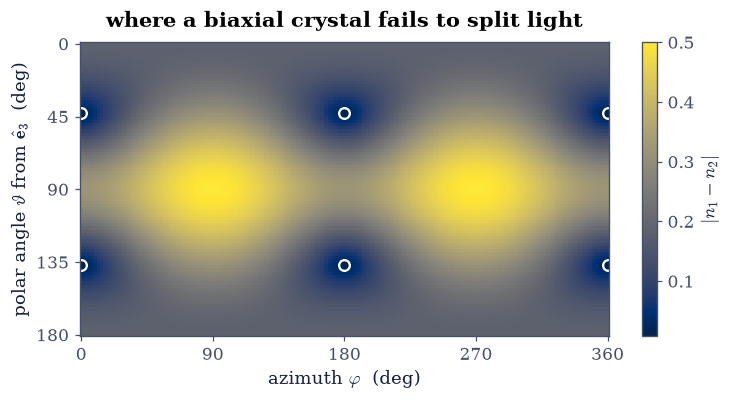
Fig. 333 The splitting \(|n_1 - n_2|\) between the two waves of the model biaxial crystal \(\mathrm{diag}(2.40, 3.00, 4.20)\), over all propagation directions, as a function of polar angle \(\vartheta\) from \(\hat{\mathbf e}_3\) and azimuth \(\varphi\). Four dark spots appear, at \(\varphi = 0\) and \(\varphi = 180^\circ\) and at \(\vartheta = 43.09^\circ\) and its supplement, marked by open circles: these are the two optic axes and their antipodes, the only directions along which this crystal does not split light. They lie in the plane of the largest and smallest principal indices, straddling \(\hat{\mathbf e}_3\), and both waves travelling along them carry the intermediate index \(n_2 = 1.732051\). A uniaxial crystal is the limit in which the two spots merge into one on the pole.#
Notebook summary#
A direction admits two waves, and finding them is a \(2\times2\) eigenproblem. Restricting the impermeability tensor to the plane perpendicular to the wave normal and diagonalizing it with
numpy.linalg.eighgave calcite’s two indices at \(30^\circ\) from the optic axis as \(1.658400\) and \(1.609865\), and both solutions satisfied the full three-dimensional Eq. 299 to \(3\times10^{-16}\), which is the check that the two-dimensional reduction is faithful (Exercise 1).Fresnel’s equation, in the form a computer can solve. The polynomial Eq. 302 solved with
numpy.rootsagreed with the eigenproblem to \(6\times10^{-14}\) everywhere more than \(5^\circ\) from the optic axis, and to only \(5\times10^{-12}\) within it, the companion-matrix route losing about half its digits exactly where the two roots nearly coincide. The textbook form Eq. 301 meanwhile diverged at its own ordinary root, reaching \(2.5\times10^{6}\) at a distance \(10^{-7}\) from it with the residue \(0.25\) the algebra predicts. Rotating tensor and wave normal together left both indices unmoved, as scalars must be (Exercise 2).Ordinary and extraordinary. Over 2001 directions the ordinary index held at \(1.6584\) with a total variation of exactly zero, while the extraordinary one traced Eq. 303 from \(1.6584\) on the axis to \(1.4864\) across it, matching the closed form to \(7\times10^{-16}\). Asked again in a frame turned by \(37^\circ\), where the engine builds no basis vector along the optic axis, the ordinary polarization still came back perpendicular to that axis to \(4\times10^{-14}\), which is what makes the label physical rather than a sorting convention (Exercise 3).
Walk-off is the \(\mathbf D\)–\(\mathbf E\) angle of §3.16, doing optics. The angle between the Poynting vector and the wave normal matched Eq. 305 to \(3\times10^{-13}\) across the sweep, vanished exactly at both ends, and peaked at \(\rho_{\max}=6.2611709^\circ\) at \(\theta^\star=41.869412^\circ\), against the closed form Eq. 306 of \(6.2611709^\circ\) at \(41.869415^\circ\). That closed form is \(\tan\alpha_{\max}=(\varepsilon_3-\varepsilon_1)/2\sqrt{\varepsilon_1\varepsilon_3}\) with \(\varepsilon_i=n_i^2\), and \(6.26^\circ\) is the number the calcite turntable of that notebook produced. Over a \(10.00\,\)mm plate it becomes \(1.0972\,\)mm of separation between the two images (Exercise 4).
Two refracted waves from one incident one. At \(30^\circ\) incidence on a calcite face cut with its optic axis \(45^\circ\) from the normal, the ordinary wave refracted at \(17.547444^\circ\) with the index \(n_o\) returned exactly by a non-diagonal laboratory-frame tensor, and the extraordinary wave at \(17.999502^\circ\) with index \(1.618077\), from a transcendental phase-matching condition solved by
brentq. The two wave normals differ by \(0.452^\circ\) and the two rays by \(4.934^\circ\), so the doubled image is mostly walk-off (Exercise 5).Two surfaces, touching once. The index surface came out as a sphere of radius \(1.6584\) with a total radial variation of \(4\times10^{-16}\), plus the spheroid Eq. 307; the wave surface, built from Poynting directions and the ray speed Eq. 313, landed on Huygens’ spheroid Eq. 308 to \(9\times10^{-16}\), with the extraordinary ray running between \(1.808\times10^{8}\) and \(2.017\times10^{8}\,\)m/s. The gap between the sheets grows fourfold per doubling of \(\theta\), a fitted exponent of \(2.000\): they touch the optic axis and cross nowhere (Exercise 6).
Wave plates out of the leftover phase. A wave normal across the optic axis has zero walk-off in both modes and indices exactly \(n_o\) and \(n_e\), so Eq. 309 applies with the measured birefringence: at the sodium D line a zero-order quarter-wave plate is \(856.5\,\)nm of calcite or \(16.17\,\mu\)m of quartz. Traced over one optical cycle and measured from its own second moments, the state out of a quarter-wave plate at \(45^\circ\) came out circular to ten decimal places with either handedness, a half-wave plate took \(\psi\) to \(-\psi\) at all eight test azimuths while leaving the state linear, and the general ellipticity followed Eq. 310. A ten-order plate is \(41\) times more wavelength-sensitive than a zero-order one (Exercise 7).
Biaxial, exactly as far as is honest. The same engine, unchanged, found the model crystal’s optic axes at \(\beta=43.088723135^\circ\) from \(\hat{\mathbf e}_3\), matching Eq. 311 to twelve digits, with both waves there carrying the intermediate index \(n_2=\sqrt3=1.7320508\). The two uniaxial crystals came back as the ends of the same family, \(\beta=0\) and \(\beta=90^\circ\) (Exercise 8).
Outlook#
Conical refraction. Exercise 8 found the optic axes and deliberately stopped. What happens along one of them is the most striking prediction in classical optics: because the wave surface has a conical point there, a narrow beam entering along an optic axis of a biaxial crystal spreads into a hollow cone inside the crystal and leaves as a bright ring. Hamilton predicted it in 1832 from the geometry of the surface alone, and Lloyd saw it in aragonite two months later, which is about as clean a case of theory preceding observation as physics has. Building it needs the biaxial ray surface, its circle of contact, and a careful convention statement first; Born and Wolf [BW99] (§15.3) give the full treatment.
Polarization as a state, and the calculus for it. Exercise 7 tracked polarization by tracing a real field and measuring the ellipse, which is honest and slow. The compact machinery is the Jones calculus, in which a state is a two-component complex vector and every plate and polarizer is a \(2\times2\) complex matrix, with the Stokes parameters and the Poincaré sphere handling partially polarized light that a single Jones vector cannot describe. This notebook leaves it out on purpose: a non-Hermitian complex \(2\times2\) object obeying a different transformation law would blur the real symmetric property tensor that §3.16 spent a whole notebook establishing. It is the right next tool, and worth meeting once the tensor is secure. The Poincaré sphere is also the Bloch sphere of §6.8 wearing different clothes, which is a coincidence worth not treating as one.
Optical activity, and the antisymmetric part. Quartz rotates the plane of polarization of light travelling along its own optic axis, where this notebook’s machinery predicts nothing at all should happen. The resolution is that \(\boldsymbol\varepsilon\) acquires a small antisymmetric imaginary part when the response is allowed to depend on \(\mathbf k\) as well as \(\omega\) (spatial dispersion), and §3.16 named that antisymmetric half as the home of the Hall effect and Faraday rotation. Everything here assumed it away with the energy argument.
Making the crystal do something. Apply a static field to a suitable crystal and \(\boldsymbol\eta\) changes with it, linearly (the Pockels effect, a rank-3 property, so by the argument in the Outlook of §3.16 it exists only in non-centrosymmetric crystals) or quadratically (the Kerr effect). A quarter-wave plate one can switch on in nanoseconds is a modulator, and it is how light is put onto a fibre. That, and the frequency doubling that phase-matching in a birefringent crystal makes possible, is nonlinear optics, which §3.15 also named as a horizon and which this course does not develop.
Where the numbers came from. Calcite’s two indices were handed to us, as the oscillator parameters were in §3.15 and the principal permittivities in §3.16. Computing them from the electronic structure of the crystal, with the tensor character intact rather than averaged away, is the subject of §8.15.
References#
Max Born and Emil Wolf. Principles of Optics: Electromagnetic Theory of Propagation, Interference and Diffraction of Light. Cambridge University Press, 7 edition, 1999. doi:10.1017/CBO9781139644181.
David J. Griffiths. Introduction to Electrodynamics. Cambridge University Press, 4 edition, 2017.
John David Jackson. Classical Electrodynamics. Wiley, 3 edition, 1998.
Wolfgang Nolting. Theoretical Physics 3: Electrodynamics. Springer, 2016.