


3.8 Maxwell’s Equations and Electromagnetic Waves#
Notebook overview#
This is the climax of the volume. Across the last seven notebooks we built the field equations one law at a time: Gauss for \(\mathbf E\) (§3.3), no monopoles for \(\mathbf B\) (§3.6), Ampère for steady currents (§3.6), and Faraday’s induction (§3.7). Three of the four were complete; one, Ampère’s law, was quietly broken the moment fields varied in time. Maxwell found the flaw, fixed it with a single new term, and in doing so turned a collection of empirical laws into one dynamical theory whose solutions travel, at a speed that turns out to be the speed of light.
We follow that path. First the inconsistency: \(\nabla\times\mathbf B=\mu_0\mathbf J\) cannot survive a changing charge density, and the charging capacitor shows it concretely, with \(\mathbf B\) circulating around a gap that no conduction current crosses. Maxwell’s fix is the displacement current \(\mu_0\varepsilon_0\,\partial_t \mathbf E\), the exact mirror of Faraday’s term: where a changing \(\mathbf B\) makes an \(\mathbf E\) (§3.7), a changing \(\mathbf E\) makes a \(\mathbf B\). That symmetry is what lets a disturbance sustain itself.
With the equations complete we take the curl of Faraday’s law, substitute Ampère–Maxwell, and watch a wave equation fall out, with speed \(v=1/\sqrt{\mu_0\varepsilon_0}\). Computing that number from the electric and magnetic constants alone, with no optics anywhere in the inputs, gives \(2.998\times10^8\,\)m/s: light is an electromagnetic wave. We then build an explicit plane wave, confirm it satisfies the wave equation numerically, animate it (the one place a moving picture is truly warranted, the iconic image of the subject), and read off its structure: \(\mathbf E\perp\mathbf B\perp\mathbf k\), in phase, with \(|\mathbf E|=c|\mathbf B|\). The Poynting vector \(\mathbf S=\tfrac1{\mu_0}\mathbf E\times\mathbf B\) tells us the wave carries energy. Finally the Lorenz gauge returns the gauge freedom of §3.6 as a tool: the right gauge choice decouples the potentials into two clean wave equations.
Everything is in SI units, with \(\mu_0=4\pi\times10^{-7}\,\)T·m/A and \(\varepsilon_0=8.854\times10^{-12}\,\)F/m. A propagating wave is genuine motion, so one figure here is animated; everything else is a still.
How to read the checks. Each exercise ends with a
validatecall against an independent fact: a displacement current equal to the conduction current, the four equations holding on a test field, \(1/\sqrt{\mu_0\varepsilon_0}\) equal to \(c\), a plane wave satisfying \(\nabla^2 E=\mu_0\varepsilon_0\,\partial_t^2 E\), the intensity \(E_0^2/2\mu_0 c\). A ✓ is strong evidence; a ✗ is a prompt to locate the discrepancy, not a verdict.A numerical-differentiation note. Several checks take first or second derivatives of a sampled field with
numpy.gradient, whose one-sided stencils at the array edges are less accurate than the centred interior stencil; we therefore validate on the interior (excluding the end points), the array-edge subtlety met since §3.6.
Theory in brief#
The inconsistency Maxwell found#
Take the divergence of the steady Ampère law \(\nabla\times\mathbf B=\mu_0\mathbf J\). The left side vanishes identically (the divergence of a curl is zero), so it demands
but charge conservation says \(\nabla\cdot\mathbf J=-\partial_t\rho\), which is nonzero wherever charge piles up. The two collide at a charging capacitor: current flows into the plates, \(\mathbf B\) circulates around the wire, yet no conduction current crosses the gap. Ampère’s law, applied to a surface bulging through the gap, gives the wrong answer.
The displacement current#
Maxwell’s fix is to add a term built from the changing field between the plates,
The new piece \(\mu_0\varepsilon_0\,\partial_t\mathbf E\) is the displacement current: a changing electric field sources \(\mathbf B\), the exact mirror of Faraday’s changing magnetic field sourcing \(\mathbf E\). In the capacitor gap \(\varepsilon_0\,\partial_t\mathbf E\) carries precisely the conduction current that was missing, and taking the divergence of Eq. 231 now reproduces charge conservation exactly.
Maxwell’s equations, complete#
Collected, the four equations are
The dynamical symmetry of the two curl equations, a changing \(\mathbf B\) making \(\mathbf E\) and a changing \(\mathbf E\) making \(\mathbf B\), is the feedback that permits a self-sustaining disturbance.
The wave equation and the speed of light#
In vacuum (\(\rho=0\), \(\mathbf J=0\)) take the curl of Faraday’s law and use the identity \(\nabla\times(\nabla\times\mathbf E)=\nabla(\nabla\cdot\mathbf E)-\nabla^2\mathbf E\). The first term vanishes (\(\nabla\cdot\mathbf E=0\)), and substituting Ampère–Maxwell for \(\nabla\times\mathbf B\) leaves
a wave equation (and the identical one for \(\mathbf B\)) with speed \(v=1/\sqrt{\mu_0\varepsilon_0}\). Evaluated from the constants,
Computed from electricity and magnetism alone, out comes the speed of light: light is an electromagnetic wave.
Plane waves and energy flux#
The simplest solutions are plane waves,
with \(\mathbf E\perp\mathbf B\perp\mathbf k\) (transverse), oscillating in phase and obeying \(|\mathbf E|=c|\mathbf B|\); the direction of \(\mathbf E\) is the polarization. The energy flux is the Poynting vector, the flux term of the local energy-conservation law that follows from Maxwell’s equations and the Lorentz force (Poynting’s theorem; Jackson [Jac98], ch. 6, carries the derivation out in full),
whose time average for a plane wave is the intensity \(\langle S\rangle=E_0^2/2\mu_0 c\). Energy, and momentum, travel with the wave.
The Lorenz gauge: gauge as a tool#
Writing the fields with potentials, \(\mathbf E=-\nabla V-\partial_t\mathbf A\) and \(\mathbf B=\nabla\times\mathbf A\) (the form forced by §3.7), Maxwell’s equations for \(V\) and \(\mathbf A\) come out coupled. Using the gauge freedom of §3.6 to impose the Lorenz condition
decouples them into two symmetric wave equations, \(\Box V=-\rho/\varepsilon_0\) and \(\Box\mathbf A=-\mu_0\mathbf J\), with \(\Box=\nabla^2-\tfrac1{c^2}\partial_t^2\) the d’Alembertian. (Jackson [Jac98], ch. 6, carries the substitution and the cancellation out in full.) The gauge freedom introduced in §3.6 is now a tool: the right choice makes the wave structure manifest. (Forward: §3.12 shows the Lorenz condition is Lorentz-invariant, gauge as structure.)
Setup#
Data and instruments only: the two vacuum constants \(\mu_0\) and \(\varepsilon_0\) that
the speed of light is computed from, the measured \(c\) they are graded against, the
series palette, and the centred second-difference operator you already built as the
five-point Laplacian in §3.4, restated here as a one-axis
call. Nothing in this notebook’s own line of argument is pre-built: the plane wave,
the four residuals, the d’Alembertian and the Poynting average are all assembled in
the exercises, out of the constants above and numpy.gradient. No randomness appears
anywhere in this notebook.
The Setup below holds this notebook’s data and instruments — nothing you are asked to build. It is collapsed so the building stays yours; expand it whenever you want the details.
Exercise 1 — The displacement current and the capacitor (worked)#
The cleanest place to see Ampère’s law fail is a charging parallel-plate capacitor. A conduction current \(I\) flows along the wire into the plates, and an Amperian loop around the wire encloses it, so \(\oint\mathbf B\cdot d\boldsymbol\ell=\mu_0 I\). But the loop bounds many surfaces, and one can be drawn to bulge between the plates, where no charge flows: through that surface the conduction current is zero (Fig. 258). The steady Ampère law Eq. 230 gives two different answers for the same loop. Maxwell’s displacement current Eq. 231 repairs it: the changing field in the gap, \(\varepsilon_0\,\partial_t\mathbf E\), carries exactly the missing current.
The capacitor here is charged by \(I=1\,\)A through plates of area \(A=0.01\,\mathrm{m}^2\), so the charge is \(Q(t)=It\) and the uniform gap field is \(E=Q/(\varepsilon_0 A)\). Maxwell’s new term, integrated over the gap, is the displacement current \(I_d=\varepsilon_0 A\,dE/dt\).
Sample \(E(t)\) over the first nanosecond of charging and differentiate it with
numpy.gradientto get \(dE/dt\), then form \(I_d=\varepsilon_0 A\,dE/dt\) (averaged over the interior, where the derivative stencil is centred).Confirm \(I_d\) equals the conduction current \(I\): the current that crosses the gap is exactly the one that flows in the wire, and the two surfaces spanning the Amperian loop agree again.
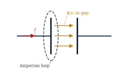
Fig. 258 A charging parallel-plate capacitor. A conduction current \(I\) (red) flows along the wire onto the left plate; between the plates no charge crosses, yet the electric field \(\mathbf E\) (amber) grows. An Amperian loop (dashed) around the wire can be spanned by a flat surface pierced by \(I\) or by a surface bulging into the gap pierced by none. Ampère’s law agrees on both only once Maxwell’s displacement current \(\varepsilon_0\,\partial_t\mathbf E\) is added, carrying the same current through the gap.#
conduction current I = 1.000000 A
displacement current I_d = 1.000000 A (= ε₀ A dE/dt)
Validation 1#
✓ the displacement current ε₀A dE/dt equals the conduction current, making ∇×B consistent [got 1 vs expected 1 (rtol=1e-06, atol=1e-09)]
True
Exercise 2 — Maxwell’s equations assembled (worked synthesis)#
With the displacement current in hand the four equations Eq. 232 are complete: Gauss (§3.3), no monopoles (§3.6), Faraday (§3.7), and the now-corrected Ampère–Maxwell law (Exercise 1). The decisive new feature is the symmetry of the two curl equations: a changing \(\mathbf B\) makes \(\mathbf E\) and a changing \(\mathbf E\) makes \(\mathbf B\), the mutual feedback that lets a disturbance propagate with no charges or currents to sustain it.
The test field is the vacuum plane wave Eq. 235, \(\mathbf E=E_0\cos(kx- \omega t)\,\hat{\mathbf y}\) and \(\mathbf B=(E_0/c)\cos(kx-\omega t)\,\hat{\mathbf z}\) with \(\omega=ck\), sampled on an \((x,t)\) grid that every later exercise reuses. That Ampère–Maxwell holds on such a source-free wave is the cleanest test that the assembled set is self-consistent — a wave needs no charges or currents, only the two curl laws feeding each other.
Sample \(E_y(x,t)\) and \(B_z(x,t)\) over two wavelengths and two periods, with \(E_0=1\,\)V/m, \(\lambda=0.5\,\)m and the phase speed \(c=1/\sqrt{\mu_0\varepsilon_0}\).
Argue the two divergence laws hold identically: \(\mathbf E\) has only a \(y\) component and \(\mathbf B\) only a \(z\) component, each depending on \(x\) alone, so \(\partial_y E_y=\partial_z B_z=0\) term by term.
Verify the two curl laws numerically on the interior (derivatives by
numpy.gradient, whose edge stencils are one-sided): Faraday \(\partial_x E_y=-\partial_t B_z\) and Ampère–Maxwell \(-\partial_x B_z=\mu_0\varepsilon_0\,\partial_t E_y\).
Gauss/no-monopole divergences vanish identically: True
Faraday ∂ₓEy = −∂ₜBz holds on the interior: True
Ampère–Maxwell −∂ₓBz = μ₀ε₀∂ₜEy holds (interior): True
Validation 2#
✓ the assembled Maxwell equations hold on the vacuum plane wave (the two curl laws numerically, the two divergences identically)
True
Exercise 3 — The wave equation and the speed of light (worked)#
Now the payoff. In vacuum, taking the curl of Faraday’s law and using \(\nabla\times(\nabla\times\mathbf E)=\nabla(\nabla\cdot\mathbf E)-\nabla^2\mathbf E\) with \(\nabla\cdot\mathbf E=0\) gives \(-\nabla^2\mathbf E=-\partial_t(\nabla\times\mathbf B)\); substituting Ampère–Maxwell \(\nabla\times\mathbf B=\mu_0\varepsilon_0\,\partial_t \mathbf E\) yields the wave equation Eq. 233, \(\nabla^2\mathbf E=\mu_0\varepsilon_0 \,\partial_t^2\mathbf E\), with speed \(v=1/\sqrt{\mu_0\varepsilon_0}\).
That speed is built from two constants measured in entirely non-optical experiments: \(\varepsilon_0\) from the force between charges (§3.1) and \(\mu_0\) from the force between currents (§3.6). Nothing about light goes into the inputs, so if \(c\) comes out, the agreement is the whole argument: light is an electromagnetic wave, one of the great unifications in physics.
Compute \(1/\sqrt{\mu_0\varepsilon_0}\) from the two Setup constants alone.
Compare it to the measured speed of light Eq. 234, as a ratio.
1/√(μ₀ε₀) = 299792457.999821 m/s
measured speed of light c = 299792458.000000 m/s
ratio = 1.000000000
Validation 3#
✓ 1/√(μ₀ε₀) equals the speed of light — light is an electromagnetic wave [got 2.99792e+08 vs expected 2.99792e+08 (rtol=1e-06, atol=1e-09)]
True
Exercise 4 — A plane wave, and the wave it makes (worked)#
The explicit plane wave Eq. 235 now has to face the equation it claims to solve. With \(E_0=1\,\)V/m, wavelength \(0.5\,\)m (so \(k=2\pi/\lambda\)) and \(\omega=ck\), the field \(E_y(x,t)=E_0\cos(kx-\omega t)\) built on the \((x,t)\) grid of Exercise 2 should satisfy the wave equation Eq. 233 exactly, and the residual it leaves behind should be nothing but the finite-difference truncation error.
Form the second derivatives \(\partial_x^2 E_y\) and \(\partial_t^2 E_y\) with the centred finite-difference stencil of Setup’s
second_deriv, the one-axis form of the five-point Laplacian you wrote in §3.4.Confirm \(\partial_x^2 E_y=\mu_0\varepsilon_0\,\partial_t^2 E_y\) on the interior, relative to the natural size of \(\partial_x^2 E_y\), and that the dispersion relation \(\omega/k=c\) holds.
Animate the wave (Fig. 259), the iconic image of the subject: \(\mathbf E\) and \(\mathbf B\) oscillating in mutually perpendicular planes while the whole pattern marches forward at \(c\).
max |∂ₓ²E − μ₀ε₀∂ₜ²E| / scale (interior) = 1.61e-11
ω/k = 299792457.999821 m/s vs c = 299792457.999821 m/s
Validation 4#
✓ the plane wave satisfies the electromagnetic wave equation with v = c [max|Δ| = 2.54943e-09 (rtol=0.001, atol=1e-09)]
✓ the dispersion relation is ω = ck [got 2.99792e+08 vs expected 2.99792e+08 (rtol=1e-06, atol=1e-09)]
True
Fig. 259 Animation of a linearly polarised plane wave travelling along \(+x\) at speed \(c\). The electric field \(\mathbf E=E_0\cos(kx-\omega t)\,\hat{\mathbf y}\) oscillates in the vertical (\(x\)–\(y\)) plane (amber) and the magnetic field \(\mathbf B=(E_0/c)\cos(kx-\omega t)\,\hat{\mathbf z}\) in the horizontal (\(x\)–\(z\)) plane (blue), in phase and mutually perpendicular. The whole transverse pattern translates rigidly at \(c\); the fields are scaled to a common height for visibility (in SI units \(|\mathbf B|=|\mathbf E|/c\)).#
Exercise 5 — The E, B, k relations (worked)#
The plane wave Eq. 235 packs three structural facts: the fields are transverse (\(\mathbf E\perp\mathbf k\) and \(\mathbf B\perp\mathbf k\)), mutually perpendicular (\(\mathbf E\perp\mathbf B\)), and locked in phase with amplitudes tied by \(|\mathbf E|=c|\mathbf B|\). Together they say the wave is a pair of sinusoids riding in orthogonal planes, the picture animated in Exercise 4.
For the wave of Exercise 2 the three directions are \(\hat{\mathbf k}=\hat{\mathbf x}\), \(\mathbf E\parallel\hat{\mathbf y}\) and \(\mathbf B\parallel\hat{\mathbf z}\).
Confirm the three perpendicularity dot products vanish.
Derive \(B_z\) from \(E_y\) via Faraday’s law — integrate \(\partial_t B_z=-\partial_x E_y\) in time (
scipy.integrate.cumulative_trapezoid) — rather than restating the constructed field, and confirm the derived wave is in phase with \(\mathbf E\) with amplitude \(E_0/c\).Confirm \(E_0/B_0=c\) (Fig. 260).
max |E·B|, |E·k|, |B·k| = 0.0e+00 (mutually perpendicular)
B derived from Faraday vs constructed B: max relative deviation = 1.10e-04 (in phase, amplitude E0/c)
E₀/B₀ = 299792457.999821 m/s vs c = 299792457.999821 m/s
Validation 5#
✓ the fields satisfy |E| = c|B| [got 2.99792e+08 vs expected 2.99792e+08 (rtol=1e-06, atol=1e-09)]
✓ E ⊥ B ⊥ k (transverse, mutually perpendicular)
✓ B derived from E via Faraday's law is in phase with E and has amplitude E₀/c [got 0.000110208 vs expected 0 (rtol=1e-06, atol=0.01)]
True
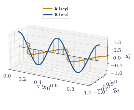
Fig. 260 A snapshot (\(t=0\)) of the plane wave’s transverse structure: \(\mathbf E\) (amber) in the \(x\)–\(y\) plane and \(\mathbf B\) (blue) in the \(x\)–\(z\) plane, drawn as field vectors along the propagation axis \(x\). The two are mutually perpendicular, perpendicular to \(\mathbf k=k\hat{\mathbf x}\), and in phase (peaks aligned); the magnetic amplitude is scaled to match the electric one for visibility (\(|\mathbf B|=|\mathbf E|/c\) in SI units).#
Exercise 6 — The Poynting vector and intensity (student)#
A wave carries energy, and the Poynting vector Eq. 236 \(\mathbf S=\tfrac1{\mu_0}\mathbf E\times\mathbf B\) measures the power per unit area it transports. For the plane wave, \(\mathbf E\times\mathbf B\) points along \(+\hat{\mathbf x}\) (the propagation direction) with magnitude \(E_0 B_0\cos^2(kx-\omega t)\), so the energy flows with the wave and pulses at twice its frequency.
Compute \(S_x(t)=\tfrac1{\mu_0}E_0 B_0\cos^2(\omega t)\) at a fixed point over one period.
Time-average it by integrating with
numpy.trapezoidand dividing by the period, and compare to the closed-form intensity \(\langle S\rangle=E_0^2/(2\mu_0 c)\) (Fig. 261).
Energy and momentum travelling with the wave are the basis of radiation pressure and of how antennas radiate (§3.10).
⟨S⟩ (time-averaged, np.trapezoid) = 1.327209e-03 W/m²
E₀²/(2μ₀c) = 1.327209e-03 W/m²
Validation 6#
✓ the time-averaged intensity is E₀²/(2μ₀c) [got 0.00132721 vs expected 0.00132721 (rtol=0.001, atol=1e-09)]
True
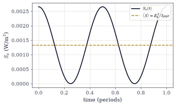
Fig. 261 The instantaneous Poynting flux \(S_x(t)=\tfrac1{\mu_0}E_0B_0\cos^2(\omega t)\) at a fixed point over one period (dark), always positive (energy flows steadily along \(+x\)) and pulsing at twice the wave frequency. Its time average (amber dashed) is the intensity \(\langle S\rangle=E_0^2/2\mu_0 c\), the steady power per unit area the wave delivers.#
Exercise 7 — The Lorenz gauge decouples the potentials (worked)#
With the potentials \(\mathbf E=-\nabla V-\partial_t\mathbf A\) and \(\mathbf B=\nabla \times\mathbf A\) (the form forced by §3.7), Maxwell’s equations become two coupled equations for \(V\) and \(\mathbf A\), tangled by cross terms. The gauge freedom of §3.6, \(\mathbf A\to\mathbf A+\nabla\chi\), is exactly the slack needed to untangle them: imposing the Lorenz condition Eq. 237 \(\nabla\cdot\mathbf A+\tfrac1{c^2} \partial_t V=0\) cancels the cross terms and leaves two symmetric wave equations, \(\Box V=-\rho/\varepsilon_0\) and \(\Box\mathbf A=-\mu_0\mathbf J\), with \(\Box=\nabla^2- \tfrac1{c^2}\partial_t^2\).
In vacuum (\(\rho=0\), \(\mathbf J=0\)) the plane-wave vector potential \(A_y=(E_0/\omega)\sin(kx-\omega t)\), which gives back \(E_y=-\partial_t A_y\), must therefore satisfy \(\Box A_y=0\) on the \((x,t)\) grid of Exercise 2. This is the second stage of the gauge arc: the freedom introduced in §3.6 turned into a tool, where the right gauge makes the wave structure fall straight out. Forward, §3.12 shows the Lorenz condition is Lorentz-invariant (gauge as structure), and Vol VI makes the gauge physical (the Aharonov–Bohm effect).
Form the d’Alembertian \(\Box A_y=\partial_x^2 A_y-\tfrac1{c^2}\partial_t^2 A_y\) with the centred finite-difference second derivatives of Setup’s
second_deriv.Confirm the residual vanishes on the interior, measured against the natural scale \(k^2|A_y|\) of each second-derivative term.
relative □A_y residual on the interior = 1.61e-11 (→ 0: □A = 0)
Validation 7#
✓ in the Lorenz gauge a vacuum plane-wave potential satisfies □A = 0 [got 1.61455e-11 vs expected 0 (rtol=1e-06, atol=0.01)]
True
Exercise 8 — The electromagnetic spectrum (student)#
Every electromagnetic wave shares the speed \(c\), so frequency and wavelength trade off through \(\lambda=c/f\). That single relation spans the entire spectrum, from kilometre-long radio waves to gamma rays smaller than a nucleus, all the same physics at different scales.
The photon energy \(E=hf\), with \(h\) Planck’s constant, is a forward pointer: that light comes in quanta of exactly that size is where Vol VI begins.
For one representative frequency in each named band (radio, microwave, infrared, visible, ultraviolet, X-ray, gamma), compute the wavelength \(\lambda=c/f\) and the photon energy \(E=hf\), and tabulate them.
Confirm \(\lambda f=c\) holds across the whole range, some fifteen decades (Fig. 262).
band f (Hz) λ (m) E = hf (eV)
radio 1.0e+06 3.00e+02 4.14e-09
microwave 1.0e+10 3.00e-02 4.14e-05
infrared 1.0e+13 3.00e-05 4.14e-02
visible 5.0e+14 6.00e-07 2.07e+00
ultraviolet 1.0e+16 3.00e-08 4.14e+01
X-ray 1.0e+18 3.00e-10 4.14e+03
gamma 1.0e+21 3.00e-13 4.14e+06
Validation 8#
✓ all electromagnetic waves satisfy λf = c across the spectrum [max|Δ| = 0 (rtol=1e-06, atol=1e-09)]
True
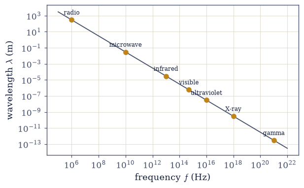
Fig. 262 The electromagnetic spectrum: wavelength against frequency on logarithmic axes, with representative points for each named band. All lie on the single line \(\lambda=c/f\) (grey), since every electromagnetic wave travels at \(c\); the bands differ only in scale, spanning some fifteen orders of magnitude from radio to gamma. The photon energy \(E=hf\) grows to the right, the quantum thread picked up in Vol VI.#
Exercise 9 — What Maxwell unified#
Stand back and take in what these four equations accomplished. Discovered piecemeal as three apparently separate subjects, electricity (Gauss), magnetism (no monopoles, Ampère) and induction (Faraday), they close, with one term added for consistency, into a single dynamical theory. And that theory’s free solutions are waves that travel at \(c\), which is the speed of light, so radio, microwaves, visible light, X-rays and gamma rays are revealed as one phenomenon at different frequencies. Few equations in physics have unified so much.
But the synthesis leaves a loose end that will not stay quiet. The wave equation Eq. 233 picks out a definite speed \(c=1/\sqrt{\mu_0\varepsilon_0}\), the same in its derivation no matter who writes it down. A speed, but relative to what? Every other wave we know travels at a fixed speed relative to a medium, and rides faster or slower for an observer moving through that medium. Maxwell’s equations name no medium and no preferred frame. That single unanswered question, a universal speed with nothing to measure it against, is the crack through which special relativity enters: the capstone (§3.12), which shows that \(\mathbf E\) and \(\mathbf B\) are one object seen from different frames, and that the Lorenz gauge condition met here is Lorentz-invariant.
The closing tally is made of numbers already measured, not of assertions: the displacement current that switched on the dynamical \(\partial_t\mathbf E\) term (Exercise 1) and the speed the completed equations predict (Exercise 3), which is the number that forces the question of frames.
List the four equations with the notebook or section where each was established.
Re-check the two measured pillars — that the displacement current of Exercise 1 equals the conduction current, and that \(1/\sqrt{\mu_0\varepsilon_0}\) of Exercise 3 equals the measured \(c\).
∇·E = ρ/ε₀ — Gauss (§3.3)
∇·B = 0 — no monopoles (§3.6)
∇×E = −∂B/∂t — Faraday (§3.7)
∇×B = μ₀J + μ₀ε₀∂E/∂t — Ampère–Maxwell (here)
displacement current measured = conduction current: True; 1/√(μ₀ε₀) = c: True
Validation 9#
✓ the two measured pillars of the synthesis hold: I_d = I (Ex 1) and 1/√(μ₀ε₀) = c (Ex 3) — light, and the question of frames that forces relativity (§3.12)
True
Notebook summary#
The displacement current Eq. 231: the charging capacitor exposed the inconsistency Eq. 230 in \(\nabla\times\mathbf B=\mu_0\mathbf J\), and \(\varepsilon_0\,\partial_t\mathbf E\) in the gap carries exactly the conduction current (Exercise 1).
Maxwell’s equations complete Eq. 232: verified on a vacuum plane wave, the two curl laws numerically and the divergences identically (Exercise 2).
Light is an electromagnetic wave Eq. 233, Eq. 234: the vacuum equations give \(\nabla^2\mathbf E=\mu_0\varepsilon_0\,\partial_t^2\mathbf E\), and \(1/\sqrt{\mu_0\varepsilon_0}=c\) from the constants alone (Exercise 3).
The plane wave Eq. 235: it satisfies the wave equation to the finite-difference floor and has \(\omega=ck\) (Exercise 4, the warranted animation); \(\mathbf E\perp\mathbf B\perp\mathbf k\), in phase, with \(|\mathbf E|=c|\mathbf B|\) (Exercise 5).
Energy flux Eq. 236: \(\langle S\rangle=E_0^2/2\mu_0 c\) by time-averaging the Poynting vector (Exercise 6).
The Lorenz gauge Eq. 237: gauge freedom as a tool, decoupling the potentials into wave equations, with \(\Box A=0\) for a vacuum wave (Exercise 7); the spectrum \(\lambda f=c\) from radio to gamma (Exercise 8); and the unification, with the “speed relative to what?” question that opens onto relativity (Exercise 9).
Outlook#
Waves in media. A refractive index \(n\), dispersion (\(n\) depending on frequency), and absorption all follow from how bound and free charges respond to the wave; reflection and refraction at an interface give the Fresnel relations.
Waveguides and cavities (§3.9). Confining a wave with conducting boundaries quantises the modes it can carry, the electromagnetic analogue of a vibrating string.
Radiation (§3.10). The displacement current also explains how accelerating charges launch these waves; the Poynting flux met here becomes radiated power.
The covariant potentials (§3.12). The Lorenz-gauge wave equations \(\Box V=-\rho/ \varepsilon_0\), \(\Box\mathbf A=-\mu_0\mathbf J\) are already relativistic in form; §3.12 makes that manifest, with gauge as structure and the field tensor \(F^{\mu\nu}\).
The speed-relative-to-what puzzle (§3.12, Vol IV). A universal \(c\) with no medium is exactly what special relativity is built to explain; that is where the volume ends.