2.6 Rigid-Body Rotation and the Spinning Top

Elementary Computational Physics

Volume II — Analytical Mechanics Notebook 2.6

The inertia tensor, Euler's equations, free precession, and the tennis-racket theorem — why a spinning body is stable about two axes and tumbles periodically about the third.

Level · advanced   •   Est. · 90–110 min

Raymond Amador v1.4.0  ·  2026-07-31  ·  CC BY 4.0 (text) / MIT (code)

Notebook overview

A rigid body has no internal degrees of freedom (every distance is frozen), so all that is left is orientation. That sounds simple, and yet a spinning body is one of the richest small systems in mechanics: a thrown phone, a tumbling wing-nut, the wobble of the Earth’s axis all live here. This notebook builds the machinery and then shows it move.

The organising idea is to change frames. The mass distribution is fixed in the body frame, so the inertia tensor \(\mathsf I\) is constant there, and we can diagonalise it once: the eigenvectors are the principal axes and the eigenvalues the principal moments \(I_1,I_2,I_3\) (the same eigenvalue problem behind normal modes in §1.5). In that frame the angular momentum is just \(\mathbf L=\mathsf I\boldsymbol\omega\) component by component, and transporting \(d\mathbf L/dt=0\) from space into the rotating body frame gives Euler’s equations: three coupled nonlinear ODEs for \(\boldsymbol\omega(t)\).

From there the physics unfolds. Torque-free, both the kinetic energy \(T\) and \(|\mathbf L|\) are conserved, so \(\boldsymbol\omega\) is pinned to the intersection of an energy ellipsoid and an angular-momentum ellipsoid: the polhode, a genuinely beautiful curve. A symmetric body (\(I_1=I_2\)) precesses freely at a rate we can predict and measure. And linearising Euler’s equations exposes the headline result, the tennis-racket (Dzhanibekov) theorem: spin is stable about the largest and smallest principal axes but unstable about the intermediate one, where the body tumbles end over end. We animate exactly that, a 3-D body spun about each axis, and then animate a symmetric top’s symmetry axis sweeping its precession cone in space.

How to read the checks. Each exercise ends with a validation that compares a computed result to an expected physical fact. A ✗ does not by itself mean the physics is wrong: it means the output didn’t match what the check expected, which may be a real error, a different-but-valid convention (a sign, a unit, an array order), or simply too tight a tolerance. Treat a ✗ as a prompt to locate the discrepancy; passing is strong evidence of correctness, not proof.

Scope. This is a working review, not a textbook chapter. For the inertia tensor, Euler’s equations, and the heavy symmetric top in full, see Nolting, Theoretical Physics 2 [Nol16], Goldstein, Poole & Safko [GPS02] (ch. 4–5), and Landau & Lifshitz, Mechanics [LL76] (§VI).

Theory in brief

The inertia tensor and principal axes

The rotational analogue of mass is the inertia tensor, defined (about the centre of mass) by

(158)\[I_{ij} = \int \rho(\mathbf r)\,\bigl(r^2\delta_{ij} - x_i x_j\bigr)\,dV ,\]

a symmetric \(3\times3\) matrix. Being symmetric, it is diagonalised by an orthogonal change of axes: its eigenvectors are the principal axes fixed in the body, and its eigenvalues the principal moments \(I_1,I_2,I_3\). Working in the principal (body) frame makes everything that follows diagonal: the same trick as resolving a coupled oscillator into normal modes (§1.5).

The conjugation behind that diagonalisation, \(\mathsf I = Q\,\mathrm{diag}(I_1,I_2,I_3)\,Q^{\mathsf T}\) with \(Q\) orthogonal, is worth naming for its own sake: it is the transformation law of a rank-2 tensor under rotation, \(I'_{ij}=Q_{ik}Q_{jl}I_{kl}\), and the inertia tensor is this course’s first specimen of the species. Whatever the axes, the trace \(I_1+I_2+I_3\) and the determinant \(I_1I_2I_3\) are invariant — the frame-independent fingerprints of the tensor, the way \(s^2\) is of an interval. The same algebra returns as the permittivity tensor of a crystal in §3.16, where the transformation law itself is put under test.

Angular momentum and kinetic energy

In the principal frame the angular momentum and rotational kinetic energy are

(159)\[\mathbf L = \mathsf I\,\boldsymbol\omega = (I_1\omega_1,\,I_2\omega_2,\,I_3\omega_3), \qquad T = \tfrac12\,\boldsymbol\omega\cdot\mathsf I\,\boldsymbol\omega = \tfrac12\bigl(I_1\omega_1^2+I_2\omega_2^2+I_3\omega_3^2\bigr).\]

Note that \(\mathbf L\) and \(\boldsymbol\omega\) are not parallel unless the body spins about a principal axis: the source of all the interesting behaviour.

Euler’s equations

In an inertial (space) frame a torque-free body conserves \(\mathbf L\): \(d\mathbf L/dt|_{\text{space}}=0\). But \(\mathsf I\) is only constant in the body frame, so we transport the derivative using \(d/dt|_{\text{space}}=d/dt|_{\text{body}}+\boldsymbol\omega\times\). With \(\mathbf L=\mathsf I\boldsymbol\omega\) this gives Euler’s equations,

(160)\[I_1\dot\omega_1 = (I_2-I_3)\,\omega_2\omega_3, \quad I_2\dot\omega_2 = (I_3-I_1)\,\omega_3\omega_1, \quad I_3\dot\omega_3 = (I_1-I_2)\,\omega_1\omega_2 ,\]

three coupled nonlinear ODEs for the body-frame angular velocity. Torque-free, they conserve both \(T\) Eq. 159 and \(|\mathbf L|\), so \(\boldsymbol\omega(t)\) is confined to the intersection of the energy ellipsoid \(\sum_i I_i\omega_i^2=2T\) and the angular-momentum ellipsoid \(\sum_i I_i^2\omega_i^2=L^2\) in \(\boldsymbol\omega\)-space (a sphere only in \(\mathbf L\)-space): the polhode.

Free precession of a symmetric top

If two moments are equal, \(I_1=I_2\), the third Euler equation gives \(\dot\omega_3=0\): the spin about the symmetry axis is constant. The other two then read \(\dot\omega_1=-\Omega\omega_2\), \(\dot\omega_2=+\Omega\omega_1\), so the transverse part of \(\boldsymbol\omega\) rotates at the free-precession rate

(161)\[\Omega = \frac{I_3-I_1}{I_1}\,\omega_3 .\]

Stability of steady rotation

Steady spin \(\boldsymbol\omega=n\,\hat{\mathbf e}_k\) about a principal axis is an exact solution. Linearising Eq. 160 about it, the transverse perturbations grow like \(e^{\sqrt{\sigma}\,t}\) with \(\sigma=-n^2(I_k-I_i)(I_k-I_j)/(I_iI_j)\), so the motion is bounded (stable) exactly when

(162)\[(I_k-I_i)(I_k-I_j) > 0 ,\]

i.e. when \(I_k\) is the largest or smallest moment. About the intermediate axis the product is negative, \(\sigma>0\), and the body tumbles: the tennis-racket / Dzhanibekov theorem.

---

Setup

We carry the principal moments as a tuple I = (I1, I2, I3) and work in the body frame. What Setup holds is data and instruments. The meters T_rot(w, I) and L_body(w, I) evaluate the closed forms Eq. 159 so the exercises can watch them not move; integrate_body(w0, I, t_eval) is the solve_ivp/DOP853 driver, and it advances \(\boldsymbol\omega(t)\) together with the orientation matrix \(\mathsf R(t)\) (body \(\to\) space) through the kinematic relation \(\dot{\mathsf R}=\mathsf R\,[\boldsymbol\omega]_\times\), because we need \(\mathsf R\) to draw the body in space for the animations — its columns are the body’s principal axes expressed in the lab frame. Finally box_polys(R, half) returns the six faces of a rectangular body rotated by \(\mathsf R\), for the 3-D renders.

This notebook’s own machinery is not here: you write Euler’s equations themselves in Exercise 2, and the driver picks them up from there.

The Setup below holds this notebook’s data and instruments — nothing you are asked to build. It is collapsed so the building stays yours; expand it whenever you want the details.

The principal axes of a rigid box are sketched in Fig. 145.

Show code cell source

Hide code cell source

import numpy as np
from scipy.integrate import solve_ivp
import matplotlib.pyplot as plt
from matplotlib.animation import FuncAnimation
from mpl_toolkits.mplot3d.art3d import Poly3DCollection

from ecp import draw, validate
from ecp.animate import show


# instrument: a conserved-quantity meter, not the lesson — the energy is the
# closed form eq-Trot already written down in the theory section, and what the
# exercises study is that it does not move, not how it is evaluated.
def T_rot(w, I):
    """Rotational kinetic energy T = (1/2) Σ I_i ω_i^2 (eq-Trot).

    Parameters
    ----------
    w : array_like
        Body angular velocity.
    I : array_like
        Principal moments.

    Returns
    -------
    float
        The rotational kinetic energy.
    """
    I1, I2, I3 = I
    return 0.5 * (I1 * w[0] ** 2 + I2 * w[1] ** 2 + I3 * w[2] ** 2)


# instrument: the companion meter to T_rot — in the principal frame L = I·ω is
# component-by-component multiplication (eq-Trot), a definition to read off
# rather than a method to build.
def L_body(w, I):
    """Angular-momentum vector in the body frame, L = I·ω (eq-Trot).

    Parameters
    ----------
    w : array_like
        Body angular velocity.
    I : array_like
        Principal moments.

    Returns
    -------
    numpy.ndarray
        The body-frame angular momentum.
    """
    I1, I2, I3 = I
    return np.array([I1 * w[0], I2 * w[1], I3 * w[2]])


# instrument: index plumbing for the kinematic relation below — the matrix that
# rewrites a cross product as a matrix product is bookkeeping, no exercise's
# lesson here.
def _skew(w):
    """Skew-symmetric matrix [ω]_x with [ω]_x v = ω × v.

    Parameters
    ----------
    w : array_like
        A 3-vector.

    Returns
    -------
    numpy.ndarray
        The 3x3 skew-symmetric matrix.
    """
    return np.array([[0.0, -w[2], w[1]], [w[2], 0.0, -w[0]], [-w[1], w[0], 0.0]])


# instrument: state packing for the driver below (ω and the nine entries of R in
# one vector) — not the lesson. It evaluates whatever `euler_eqs` is bound to
# when it runs: the one you write in Exercise 2, since Python looks the name up
# at call time, not at definition time.
def _rigid_rhs(_t, y, I):
    """Combined state derivative for ω and the orientation R (dR/dt = R·[ω]_x)."""
    w = y[:3]
    R = y[3:].reshape(3, 3)
    dw = euler_eqs(_t, w, I)
    dR = R @ _skew(w)
    return np.concatenate([dw, dR.ravel()])


# instrument: the solve_ivp/DOP853 driver — calling a library integrator is
# plumbing, not this notebook's craft. It carries the orientation R alongside ω
# so the body can be drawn in space, and through `_rigid_rhs` it advances your
# Exercise 2 `euler_eqs`.
def integrate_body(w0, I, t_eval, R0=None):
    """Integrate angular velocity and body-to-space orientation together.

    Advances ω(t) by Euler's equations and the rotation R(t) alongside it, so
    the body can be drawn in space.

    Parameters
    ----------
    w0 : array_like
        Initial body angular velocity.
    I : array_like
        Principal moments.
    t_eval : numpy.ndarray
        Output times.
    R0 : numpy.ndarray, optional
        Initial orientation (default identity).

    Returns
    -------
    tuple
        The angular-velocity history and the orientation history.
    """
    if R0 is None:
        R0 = np.eye(3)
    y0 = np.concatenate([np.asarray(w0, float), R0.ravel()])
    sol = solve_ivp(
        _rigid_rhs,
        (t_eval[0], t_eval[-1]),
        y0,
        args=(I,),
        method="DOP853",
        t_eval=t_eval,
        rtol=1e-11,
        atol=1e-13,
    )
    w = sol.y[:3]
    R = sol.y[3:].T.reshape(-1, 3, 3)
    return w, R


# data: the rectangular body for the 3-D renders — face vertex order and the
# six face colours, drawn from the box's half-extents.
_BOX_FACES = [
    [0, 1, 2, 3],
    [4, 5, 6, 7],
    [0, 1, 5, 4],
    [2, 3, 7, 6],
    [1, 2, 6, 5],
    [0, 3, 7, 4],
]
FACE_COLORS = ["#c0851a", "#e3b667", "#46506b", "#7b86a6", "#16213e", "#3a4a6a"]


# instrument: a rendering scaffold — turning half-extents into six rotated face
# polygons is drawing, not physics.
def box_polys(R, half):
    """The six face polygons of a box rotated by an orientation matrix.

    For rendering the spinning body's faces in 3-D.

    Parameters
    ----------
    R : numpy.ndarray
        Orientation matrix.
    half : array_like
        Box half-extents.

    Returns
    -------
    list of numpy.ndarray
        The six face-vertex arrays.
    """
    hx, hy, hz = half
    corners = np.array(
        [
            [-hx, -hy, -hz],
            [hx, -hy, -hz],
            [hx, hy, -hz],
            [-hx, hy, -hz],
            [-hx, -hy, hz],
            [hx, -hy, hz],
            [hx, hy, hz],
            [-hx, hy, hz],
        ]
    )
    pts = (R @ corners.T).T
    return [pts[idx] for idx in _BOX_FACES]

Exercise 1 — The inertia tensor and principal axes

Everything begins with \(\mathsf I\). For a body aligned with its principal axes the tensor is diagonal and the moments are the familiar integrals; for a uniform rectangular box of full side lengths \((a,b,c)\) and mass \(m\), \(I_1=\tfrac{m}{12}(b^2+c^2)\) and cyclic. But a body handed to us in an arbitrary orientation has a full (non-diagonal) \(\mathsf I\), and diagonalising it Eq. 158 recovers the same three principal moments as eigenvalues. That is the eigenvalue problem of §1.5 wearing a different hat.

1. Compute the analytic principal moments of a uniform box \((a,b,c)\) with \(a>b>c\), so \(I_1<I_2<I_3\) (the geometry of Fig. 145).

2. Build a non-aligned inertia matrix \(\mathsf I'=\mathsf Q\,\mathrm{diag}(I_1,I_2,I_3)\,\mathsf Q^\top\) for some rotation \(\mathsf Q\) (numpy.linalg.qr on a seeded random matrix), diagonalise it with numpy.linalg.eigvalsh, and confirm the eigenvalues are the analytic moments.

analytic principal moments: I1=0.17667, I2=0.34667, I3=0.49667
eigenvalues of the misaligned tensor: 0.17667, 0.34667, 0.49667

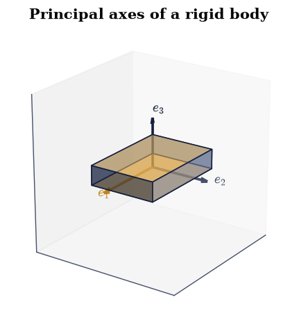
Fig. 145 A rigid rectangular body (a “book”, side lengths \(a>b>c\)) with its three principal axes through the centre of mass: \(\hat{\mathbf e}_1\) (amber, along the longest side, smallest moment \(I_1\)), \(\hat{\mathbf e}_2\) (the intermediate axis, moment \(I_2\)), and \(\hat{\mathbf e}_3\) (along the shortest side, largest moment \(I_3\)). In this principal frame the inertia tensor Eq. 158 is diagonal, \(\mathrm{diag}(I_1,I_2,I_3)\). The intermediate axis \(\hat{\mathbf e}_2\) is the unstable one of Exercise 5.

Validation 1 — principal moments match the analytic box result

Diagonalising the arbitrarily-oriented inertia tensor must return exactly the three analytic box moments: orientation cannot change the eigenvalues.

✓  principal moments match the analytic box result   [max|Δ| = 3.88578e-16 (rtol=1e-10, atol=1e-09)]

True

Exercise 2 — Euler’s equations: torque-free integration

With the principal frame in hand, the dynamics are Euler’s three equations Eq. 160. For a generic asymmetric top (\(I_1\neq I_2\neq I_3\)) they are nonlinear and the components \(\omega_i(t)\) trade energy back and forth in a periodic dance, but two combinations never change: the kinetic energy \(T\) and the magnitude \(|\mathbf L|\).

Written out for the code, each equation is one line: divide Eq. 160 through by the moment on its left, and \(\dot\omega_1=(I_2-I_3)\omega_2\omega_3/I_1\) with its two cyclic partners is the whole right-hand side. Note the cyclic pattern \(1\to2\to3\to1\) in both the index and the moment differences — the commonest way to get this wrong is to break it. The Setup’s integrate_body will hand your function the current \(\boldsymbol\omega\) and the moments and ask for \(d\boldsymbol\omega/dt\), in the signature (t, w, I) that scipy.integrate.solve_ivp expects (the time argument is unused: a torque-free body has no explicit time dependence).

1. Write euler_eqs(t, w, I), the body-frame right-hand side \(d\boldsymbol\omega/dt\) of Euler’s equations Eq. 160 for a torque-free body, returning the three components as a NumPy array. Write this one yourself — the implementation is the lesson.

2. Integrate \(\boldsymbol\omega(t)\) for an asymmetric top from a generic start with integrate_body (a scipy.integrate.solve_ivp/DOP853 wrapper on a dense t_eval, which advances the equations you just wrote) and plot the three components (Fig. 146).

3. Track \(T(t)\) and \(|\mathbf L(t)|\) (the Setup’s T_rot and L_body meters) and confirm they are conserved.

T:    2.820000 → 2.820000
|L|:  4.180909 → 4.180909

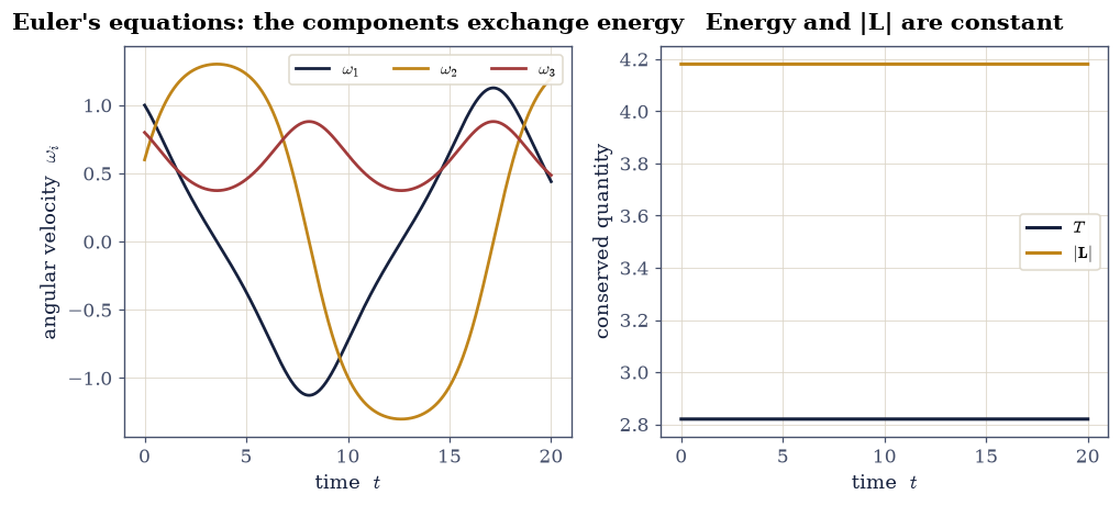
Fig. 146 Torque-free motion of an asymmetric top (\(I=(2,3,4)\)) from a generic initial spin. Left: the body-frame angular-velocity components \(\omega_1,\omega_2,\omega_3\) from Euler’s equations Eq. 160 exchange energy periodically. Right: the kinetic energy \(T\) Eq. 159 and the angular-momentum magnitude \(|\mathbf L|\) stay constant to the integrator tolerance — the two invariants that confine the motion to the polhode of Exercise 3.

Validation 2 — energy and \(|\mathbf L|\) are conserved (torque-free)

The two invariants of free rigid-body motion: \(T\) and \(|\mathbf L|\) may drift only at the integrator’s tolerance.

✓  rotational energy conserved (torque-free)   [max relative drift = 1.95273e-13 (limit 1e-06)]
✓  |L| conserved (torque-free)   [max relative drift = 9.3897e-14 (limit 1e-06)]

True

Exercise 3 — The polhode (worked)

The two invariants have a gorgeous geometric meaning. In \(\boldsymbol\omega\)-space, \(T=\text{const}\) is an ellipsoid (semi-axes \(\sqrt{2T/I_i}\)) and \(|\mathbf L|=\text{const}\) is a second ellipsoid; \(\boldsymbol\omega(t)\) must lie on both, so it traces their intersection: the polhode. Poinsot’s construction: the tip of \(\boldsymbol\omega\) rolls along this closed curve on the energy ellipsoid. We plot it and verify, point by point, that the trajectory never leaves either constraint surface.

This is a worked exercise; you build the body-in-space animation in Exercise 6.

Your task.

1. Plot the energy ellipsoid and overlay the polhode \(\boldsymbol\omega(t)\) from Exercise 2 (Fig. 147).

2. Confirm every point of the trajectory sits on both the energy ellipsoid (\(T=T_0\)) and the angular-momentum ellipsoid (\(|\mathbf L|=L_0\)).

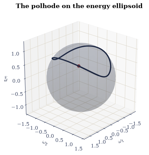
Fig. 147 The polhode for the asymmetric top of Exercise 2 (\(I=(2,3,4)\)). The angular velocity \(\boldsymbol\omega(t)\) (blue curve) is pinned to the intersection of the energy ellipsoid \(\sum_i I_i\omega_i^2=2T\) (translucent surface) and the angular-momentum ellipsoid \(\sum_i I_i^2\omega_i^2=L^2\); the tip of \(\boldsymbol\omega\) rolls along this closed curve (Poinsot’s construction). Energy and \(|\mathbf L|\) conservation are the two surfaces, and the polhode is where they meet.

Validation 3 — \(\boldsymbol\omega\) stays on the energy ellipsoid and momentum ellipsoid

The defining property of the polhode: every sampled \(\boldsymbol\omega(t)\) satisfies both \(T(\boldsymbol\omega)=T_0\) and \(|\mathbf L(\boldsymbol\omega)|=L_0\): it lives on the intersection of the two ellipsoids.

✓  ω stays on the energy ellipsoid (T constant)   [max|Δ| = 5.50671e-13 (rtol=1e-06, atol=1e-09)]
✓  ω stays on the angular-momentum ellipsoid (|L| constant)   [max|Δ| = 3.92575e-13 (rtol=1e-06, atol=1e-09)]

True

Exercise 4 — Symmetric-top free precession

Give the body an axis of symmetry, \(I_1=I_2\), and Euler’s equations simplify dramatically: \(\omega_3\) is locked constant, and the transverse part \((\omega_1,\omega_2)\) rotates rigidly at the free-precession rate \(\Omega\) Eq. 161. This is the wobble of a thrown frisbee or a slightly-off spin. We integrate, confirm \(\omega_3\) is constant, and measure \(\Omega\) from the phase of the transverse motion to compare with the prediction.

1. Set \(I_1=I_2\), integrate with integrate_body (solve_ivp/DOP853, driving the euler_eqs you wrote in Exercise 2), and check \(\omega_3\) is constant.

2. Measure the precession rate from the phase of \((\omega_1,\omega_2)\) (numpy.unwrap of numpy.arctan2, slope by numpy.polyfit) and compare to \(\Omega=(I_3-I_1)/I_1\cdot\omega_3\) (Fig. 148).

ω₃: constant? ptp = 0.00e+00  (value 3.0000)
precession rate: measured Ω = 1.800000, predicted = 1.800000

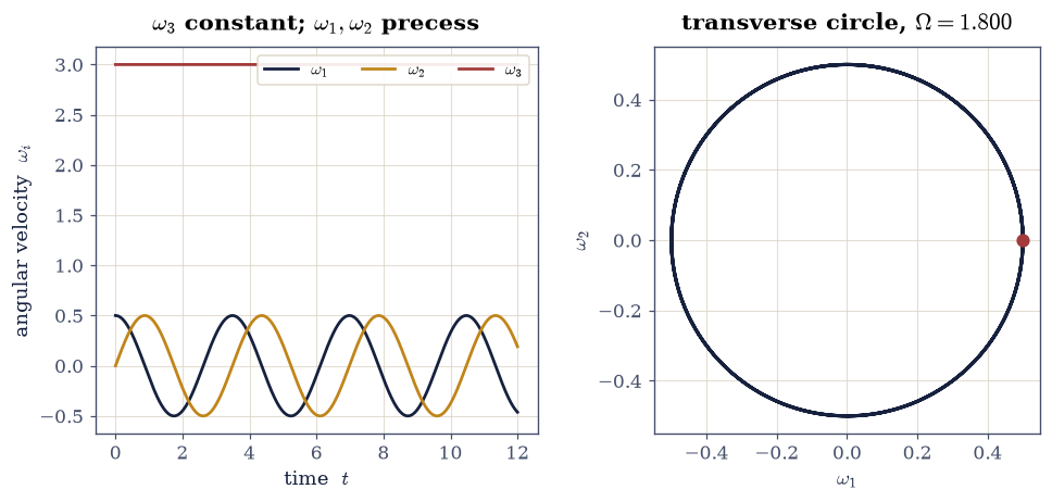
Fig. 148 Free precession of a symmetric top (\(I_1=I_2=1\), \(I_3=1.6\)). Left: the spin \(\omega_3\) (red) is exactly constant while the transverse components \(\omega_1,\omega_2\) (blue, orange) oscillate in quadrature — the transverse vector rotates rigidly. Right: \((\omega_1,\omega_2)\) traces a circle whose angular rate is the free-precession rate \(\Omega=(I_3-I_1)/I_1\,\omega_3\) Eq. 161, here measured from the phase slope to better than \(10^{-3}\).

Validation 4 — the free-precession rate is \((I_3-I_1)/I_1\cdot\omega_3\)

Two facts about the symmetric top: \(\omega_3\) is exactly constant, and the transverse precession rate matches the closed form Eq. 161.

✓  free precession rate is (I₃−I₁)/I₁·ω₃   [got 1.8 vs expected 1.8 (rtol=0.001, atol=1e-09)]
✓  ω₃ is constant for the symmetric top   [got 0 vs expected 0 (rtol=1e-06, atol=1e-09)]

True

Exercise 5 — The tennis-racket theorem (worked animation, centrepiece)

Here is the showpiece. Take a fully asymmetric body (\(I_1<I_2<I_3\)) and spin it about each principal axis with a tiny transverse nudge. The stability criterion Eq. 162 predicts a sharp dichotomy: about the smallest and largest axes the nudge stays small forever (stable spin, a barely-visible wobble), but about the intermediate axis it explodes: the body flips end over end, again and again. This is the tennis-racket / Dzhanibekov theorem, the reason a flipped phone or a tumbling wing-nut in orbit periodically reverses. We animate all three at once, every run driven by the euler_eqs you wrote in Exercise 2 — so the tumbling below is your equations of motion talking.

This is the worked animation; you build the body-in-space precession animation in Exercise 6.

transverse growth (relative to spin):
  about min axis  (I1): 0.0385   (stable)
  about mid axis  (I2): 1.1364   (UNSTABLE)
  about max axis  (I3): 0.0289   (stable)

Once Loop Reflect

Fig. 149 Animation of a rigid body (a “book”, \(I_1<I_2<I_3\)) spun about each principal axis with a tiny perturbation. About the smallest axis \(\hat{\mathbf e}_1\) (left) and largest axis \(\hat{\mathbf e}_3\) (right) the spin is stable — the body merely rotates with a faint wobble. About the intermediate axis \(\hat{\mathbf e}_2\) (centre) it is unstable: the body tumbles and periodically flips end over end. This is the tennis-racket / Dzhanibekov theorem, the stability criterion Eq. 162 made visible.

Validation 5 — stable about the extreme axes, unstable about the intermediate

The tennis-racket theorem as a number: the perturbation stays tiny for spins about the smallest and largest moments, but grows to order unity (the body tumbles) for the intermediate axis: exactly the sign of Eq. 162.

✓  spin is stable about the extreme axes, unstable about the intermediate axis   [growth: min 0.038, mid 1.136, max 0.029]

True

Exercise 6 — Body orientation in space (student-implemented animation)

Euler’s equations live entirely in the body frame, but to watch a top precess we need its orientation in the lab frame. That is the role of the rotation matrix \(\mathsf R(t)\) integrated in integrate_body via \(\dot{\mathsf R}=\mathsf R\,[\boldsymbol\omega]_\times\). For the symmetric top, the symmetry axis \(\hat{\mathbf e}_3(t)=\mathsf R(t)\,\hat{\mathbf z}\) sweeps a cone about the (space-fixed) angular momentum \(\mathbf L\): the visual signature of free precession. A subtlety worth checking: a numerically integrated \(\mathsf R\) can drift away from being a true rotation, so we confirm it stays orthonormal, \(\mathsf R^\top\mathsf R=\mathsf I\).

This is the student-implemented animation. The orientation integration is given; you build the player and make the precession cone visible.

1. Integrate \(\mathsf R(t)\) for the symmetric top with integrate_body (done for you below, still driving your Exercise 2 euler_eqs) and form the symmetry axis \(\hat{\mathbf e}_3(t)\) and the space-fixed \(\mathbf L\).

2. Build the animation of the body axes in space: at minimum the symmetry axis tracing its cone around \(\mathbf L\) — then plt.close(fig) and end with ecp.animate.show(anim). There are many valid ways to draw it.

3. Confirm \(\mathsf R(t)\) stays a proper rotation, \(\max|\mathsf R^\top\mathsf R-\mathsf I|\approx0\).

A ✗ on the final check is about the orientation integration / orthonormality, not the drawing: any correct animation of the same data is fine. If it fails, tighten the integrator tolerances or renormalise \(\mathsf R\) (Gram–Schmidt) and note why.

max |RᵀR − I| over the run = 2.60e-11  (no renormalisation needed)

Once Loop Reflect

Fig. 150 Animation of a symmetric top’s free precession in the lab frame (\(I_1=I_2=1\), \(I_3=1.6\)). The body’s symmetry axis \(\hat{\mathbf e}_3\) (red) sweeps a cone (its tip traces the grey circle) about the space-fixed angular momentum \(\mathbf L\) (amber, vertical), while the transverse body axes \(\hat{\mathbf e}_1,\hat{\mathbf e}_2\) (blue, orange) carry the spin. This is the same motion as Exercise 4’s transverse circle, now seen as the orientation of the body in space — reconstructed by integrating \(\dot{\mathsf R}=\mathsf R[\boldsymbol\omega]_\times\).

Validation 6 — the integrated orientation stays a proper rotation

The orientation reconstruction is only trustworthy if \(\mathsf R(t)\) remains a rotation: \(\mathsf R^\top\mathsf R=\mathsf I\). With the tight integrator tolerances it holds to well within \(10^{-6}\), so no renormalisation is needed here.

✓  the integrated orientation stays a proper rotation (RᵀR=I)   [got 2.60006e-11 vs expected 0 (rtol=1e-06, atol=1e-06)]

True

Notebook summary

• The inertia tensor and its principal axes; torque-free Euler’s equations integrated with \(|\mathbf L|\) conserved; the polhode traced on the inertia ellipsoid.

• Symmetric-top free precession (\(\omega_3\) constant); the tennis-racket theorem (the intermediate-axis instability) as the centrepiece; and the body’s orientation reconstructed in space.

Outlook

• The heavy symmetric top. Add a gravity torque and the free precession of Exercise 4 acquires a slow precession of the symmetry axis about the vertical plus a nutation (nodding); the cleanest treatment uses the Euler angles and the conserved \(L_z\), \(L_3\), and \(E\) (Goldstein ch. 5).

• Euler angles and gimbal lock. The full configuration space of orientations is \(SO(3)\); the Euler-angle chart has a coordinate singularity (gimbal lock) that integrating \(\mathsf R\) (or a quaternion) directly, as we did, neatly avoids.

• The Dzhanibekov effect in orbit. The intermediate-axis tumbling of Exercise 5 is the famous “tumbling wing-nut” filmed on the ISS: the tennis-racket theorem in microgravity.

• Chandler wobble. The Earth is an oblate symmetric top with \((I_3-I_1)/I_1\approx1/305\); Eq. 161 predicts a free-precession period of order a year: the observed Chandler wobble of the pole.

References

[GPS02]

Herbert Goldstein, Charles P. Poole, and John L. Safko. Classical Mechanics. Pearson, 3 edition, 2002.

[LL76]

L. D. Landau and E. M. Lifshitz. Mechanics. Volume 1 of Course of Theoretical Physics. Butterworth–Heinemann, 3 edition, 1976.

[Nol16]

Wolfgang Nolting. Theoretical Physics 2: Analytical Mechanics. Springer, 2016.

Take this notebook with you

Use the download button (↓) in the toolbar above to save this notebook and run it yourself. The published notebooks ship without worked solutions; if you would like the reference solutions — to teach from or to check your own work — get in touch: hello@ramador.me.