


5.6 The Classical Ideal Gas: Phase-Space Volume, Chemical Potential, and the Fundamental Relation#
Notebook overview#
§5.4 built the microcanonical ensemble for a discrete system — spins we could count one configuration at a time — and §5.5 reassured us the ensemble averages it computes are the ones a real system measures. Now we pay the price of going continuous, and the price is the whole point. A gas has no microstates to count: its phase space is a continuum, so its multiplicity is a volume in the \(6N\)-dimensional space of all positions and momenta. Computing that volume honestly — the volume of a ball in three thousand dimensions, regulated by a \(\Gamma\) function — is real work, and this notebook does it rather than wave it away. The reward is everything: from that one integral, all of equilibrium thermodynamics follows by differentiation. The ideal gas law, the energy, the chemical potential, and the master equation \(dU=T\,dS-P\,dV+\mu\,dN\) are each a derivative of a single entropy.
The classical route is harder than the binomial coefficient of §5.4, and that is correct: we earn the
equation of state by doing the integral, not by assuming the answer. The arsenal carries us
through. The phase-space volume overflows any float, so we live in log space with
scipy.special.gammaln (the lesson of §5.3 and §0.1, now in \(3N\) dimensions). The worry that the
answer depends on an arbitrary shell thickness dissolves through concentration of measure —
the astonishing high-dimensional fact that almost all of a ball sits in a whisker-thin skin near
its surface, a geometric cousin of the large-\(N\) sharpening of §5.3. And the Maxwell–Boltzmann
velocity law turns out to be the shadow of the energy sphere projected onto one axis: a Gaussian
by the same central-limit mechanism of §5.3, revealing the geometric origin of the Boltzmann factor
\(e^{-mv^2/2kT}\).
We will (1) build the phase-space volume, (2) prove the shell and the ball carry the same entropy, (3,4) extract \(E=\tfrac32NkT\) and \(PV=NkT\) from first principles, (5) compute the chemical potential, (6) assemble the fundamental relation, (7) derive Maxwell’s 1860 law as a sphere projection, (8) meet the Gibbs paradox — the one place classical counting genuinely fails, an honest cliffhanger to Volume VII — and (9) extend equipartition. We work in units \(m=h=k_B=1\) throughout, stated wherever it matters.
How to read the checks. Each exercise closes with a
validatecall against an independent fact: the \(V^N\times\)(\(3N\)-ball) volume; the outer-shell concentration and shell–ball agreement; \(E=\tfrac32NkT\) and \(PV=NkT\) from \(\partial S/\partial E\) and \(\partial S/\partial V\); the chemical potential \(\mu=-T\,\partial S/\partial N\); the fundamental relation as a numerical identity; a velocity component Gaussian with variance \(kT/m\); the Gibbs factor restoring extensivity; and classical equipartition. A ✓ is strong evidence; a ✗ is a prompt to locate the discrepancy.Scope. The classical microcanonical ideal gas and the fundamental relation. Thermodynamic potentials, Legendre transforms, and Maxwell relations are §5.7; the grand canonical ensemble (and \(\mu\)’s starring role) later in the volume; the absolute entropy (Sackur–Tetrode) and the origin of the \(1/N!\) are Volume VII. See Schroeder, An Introduction to Thermal Physics; Kardar, Statistical Physics of Particles; Maxwell (1860); and §5.4, §5.3, §0.1.
Theory in brief#
The phase-space volume of a classical system#
For a classical system the microcanonical multiplicity is a phase-space volume, not a count. For \(N\) free particles in a box of volume \(V\) with energy \(\le E\), the accessible region is \(V^N\) (positions) times the volume of the momentum ball of radius \(\sqrt{2mE}\) in \(3N\) dimensions. The \(n\)-ball volume is \(V_n(R)=\pi^{n/2}R^n/\Gamma(n/2+1)\), so
(the result of which is derived in every standard classical statistical mechanics course; as it
is a routine pencil-and-paper exercise, and emphatically not per se of computational interest,
we do not reproduce the derivation here — Schroeder, An Introduction to Thermal Physics,
§2.5, carries it out in full). The \(1/h^{3N}\) makes \(\Sigma\) dimensionless (\(h\) sets
the size of a phase-space cell — its value is fixed by quantum mechanics, but it only shifts the
entropy by an additive constant), and the
\(1/N!\) is the Gibbs indistinguishability factor (also quantum in origin; its role is Exercise
8). We compute \(\ln\Sigma\) with scipy.special.gammaln because \(\Sigma\) overflows (§5.3/§0.1, now
in \(3N\) dimensions).
Shell versus ball, and concentration of measure#
The microcanonical ensemble lives on the energy shell (\(E\) in \([E,E+\Delta E]\)), of volume \(g(E)\Delta E\) with the density of states \(g=\partial\Sigma/\partial E\). Does the entropy depend on the arbitrary thickness \(\Delta E\), or on shell-versus-ball? At large \(N\), no — because of concentration of measure: in high dimensions almost all of a ball’s volume lies in a thin outer shell,
so \(\ln\Sigma\approx\ln(g\,\Delta E)\) to \(O(\ln N)\), and the entropy per particle is the same whichever we use. This is the geometric cousin of the large-\(N\) sharpening of §5.3.
Entropy, the equations of state, and the chemical potential#
With \(S=k\ln\Omega\) (§5.4) the derivatives give everything,
the caloric and thermal equations of state — the ideal gas law derived, not assumed. The third derivative is the chemical potential, the energy cost of adding a particle,
negative for a dilute classical gas, and the quantity that governs particle exchange (central to the grand canonical ensemble). Assembling all three derivatives gives the fundamental thermodynamic relation,
the master equation of equilibrium thermodynamics — it packages the first and second laws and defines \(T,P,\mu\) as entropy’s conjugate slopes. §5.7 builds the potentials on it.
Maxwell–Boltzmann as the shadow of the sphere#
With total kinetic energy fixed, the \(3N\) velocity components lie uniformly on a sphere of radius \(\sqrt{2E/m}\) in \(3N\) dimensions. The marginal of a single component is the projection of that uniform sphere onto one axis — uniform for \(n=3\) (Archimedes), and Gaussian as \(n\) grows,
the Maxwell–Boltzmann law (Maxwell 1860, the first statistical law in physics). The speed obeys \(f(v)\propto v^2 e^{-mv^2/2kT}\) with \(\langle v\rangle=\sqrt{8kT/\pi m}\) and \(v_{\rm rms}=\sqrt{3kT/m}\). This is the geometric origin of the Boltzmann factor: the shadow of a high-dimensional sphere (the §5.3 Gaussian again).
The Gibbs paradox: where classical counting fails#
Without the \(1/N!\), the entropy is not extensive: combining two boxes of the same gas predicts a spurious increase,
The \(1/N!\) restores extensivity. But indistinguishability, and the \(h\) that fixes the absolute entropy (Sackur–Tetrode), are quantum in origin: classical mechanics gives the form of the entropy and every difference, but cannot fix its absolute scale or justify the \(1/N!\) on its own. We defer that to Volume VII — classical mechanics taken exactly as far as it honestly goes. The entropy of mixing of different gases, by contrast, is real: \(\Delta S=2Nk\ln 2\), the \(-k\sum x\ln x\) of §5.3.
Setup#
Data only: the unit convention \(m=h=k_B=1\), the worked state \((N,V,E)\) that every
derivative below is taken around, and the series palette. There are no instruments —
nothing in this notebook’s line of argument arrives pre-built. The machinery is yours:
the log phase-space volume \(\ln\Sigma\) is built in Exercise 1, the log density of states
\(\ln g\) in Exercise 2, and the uniform sampler on the energy sphere in Exercise 7; every
other quantity here is a finite difference or a numpy.gradient of those.
The Setup below holds this notebook’s data and instruments — nothing you are asked to build. It is collapsed so the building stays yours; expand it whenever you want the details.
Exercise 1 — The phase-space volume of the ideal gas (worked)#
We begin by building the multiplicity honestly, because everything rests on it. For a gas there is
nothing to count one-by-one: a microstate is a point in the \(6N\)-dimensional phase space of all
positions and momenta, and the microcanonical multiplicity is the volume of the accessible
region. That region factorizes (Fig. 430): each particle’s position ranges freely over
the box, giving \(V^N\); and the momenta, constrained by \(\sum p_i^2/2m\le E\), fill a ball of
radius \(\sqrt{2mE}\) in \(3N\) dimensions. The volume of an \(n\)-ball is \(V_n(R)=\pi^{n/2}R^n/
\Gamma(n/2+1)\) — the \(\Gamma\) function is what regulates “the volume of a ball” once \(n\) is large
— so the whole phase-space volume is Eq. 410. Two prefactors appear that classical
mechanics cannot itself justify: \(1/h^{3N}\), which makes \(\Sigma\) dimensionless (\(h\) is the size
of a phase-space cell), and the Gibbs factor \(1/N!\) for indistinguishability. Both are quantum in
origin; we flag them now and resolve the \(1/N!\) in Exercise 8. As §5.3 warned, the volume itself
overflows instantly — in \(3N=3000\) dimensions it has thousands of digits — so we compute
\(\ln\Sigma\) with scipy.special.gammaln.
Two independent facts pin the assembled expression down. The \(\Gamma\)-regulated ball formula must reduce to elementary geometry when there is only one particle: at \(N=1\) the momentum ball is an ordinary \(3\)-ball, so \(\Sigma=V\cdot\tfrac43\pi(2mE)^{3/2}\) with no \(\Gamma\) function anywhere (and no Gibbs factor, since \(1!=1\)). And the raw \(\Sigma\) must overflow: a number with thousands of digits has no float representation, while its logarithm is an ordinary few-thousand.
Part a) Write ln_Sigma(E, V, N, gibbs=True), the log phase-space volume
Eq. 410: \(N\ln V\) for the positions, \(\tfrac{3N}{2}\ln(2\pi mE)-
\ln\Gamma(\tfrac{3N}{2}+1)\) for the \(3N\)-dimensional momentum ball, \(-3N\ln h\) for the
phase-space cell, and \(-\ln N!\) for the Gibbs factor under a gibbs switch (Exercise 8 turns it
off). Every factorial and every \(\Gamma\) goes through scipy.special.gammaln — the function is
never allowed to form \(\Sigma\) itself. Write this one yourself — the implementation is the
lesson.
Part b) Assemble the same number a second time and independently, piece by piece from \(N\ln V\), the ball’s \(\pi^{3N/2}R^{3N}/\Gamma(\tfrac{3N}{2}+1)\) with \(R=\sqrt{2mE}\), and the \(1/N!\); confirm the two routes agree at \(10^{-12}\).
Part c) Evaluate the \(N=1\) case (Gibbs factor off) against the elementary \(V\cdot\tfrac43\pi(2mE)^{3/2}\) computed directly, and confirm they are the same number.
Part d) Confirm that \(\exp(\ln\Sigma)\) overflows to infinity while \(\ln\Sigma\) itself stays finite, and report how many digits the raw volume would have.
state: N=1000, V=1000.0, E=1500.0 (units m=h=k=1)
ln Σ = 5247.8671   (piecewise check: 5247.8671)
N=1 anchor: ln Σ = 20.349719  vs elementary V·(4/3)π(2mE)^(3/2) = 20.349719
raw Σ = exp(ln Σ) overflows a float: True  (it has ~2279 digits)
/tmp/ipykernel_3921/982139788.py:55: RuntimeWarning: overflow encountered in exp
  f"raw Σ = exp(ln Σ) overflows a float: {np.isinf(np.exp(ln_sigma))}  (it has ~{int(ln_sigma/np.log(10))} digits)"
Validation 1#
✓  the ideal-gas phase-space volume is the V^N × (3N-ball) expression   [got 5247.87 vs expected 5247.87 (rtol=1e-12, atol=1e-09)]
✓  the Γ-regulated ball formula reduces to the elementary (4/3)πR³ ball at N=1   [got 20.3497 vs expected 20.3497 (rtol=1e-12, atol=1e-09)]
✓  the raw phase-space volume overflows a float; its logarithm via gammaln does not
/tmp/ipykernel_3921/171223410.py:14: RuntimeWarning: overflow encountered in exp
  np.isinf(np.exp(ln_sigma)) and np.isfinite(ln_sigma),
True
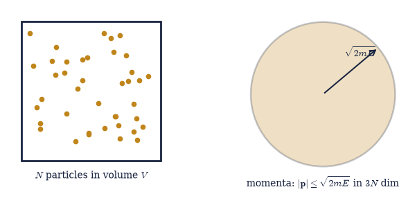
Fig. 430 The two factors of the ideal-gas phase-space volume. Left: \(N\) point particles range freely over the box of volume \(V\), contributing \(V^N\) to the accessible volume (positions). Right: with energy fixed, the \(3N\) momentum components are confined to a ball of radius \(\sqrt{2mE}\) in \(3N\) dimensions, contributing \(\pi^{3N/2}R^{3N}/\Gamma(\tfrac{3N}{2}+1)\) (momenta). The full microcanonical multiplicity is their product, divided by \(h^{3N}N!\). There is nothing to count — only a volume to integrate, and that integral is the whole classical cost.#
Exercise 2 — Concentration of measure: shell versus ball (worked)#
A worry must be dealt with before we differentiate, and dealing with it teaches a remarkable fact about high-dimensional space. The microcanonical ensemble strictly lives on the energy shell — energies in \([E,E+\Delta E]\) — not the filled ball of energies \(\le E\). Does the entropy then depend on the arbitrary thickness \(\Delta E\), or on which we use? The resolution is concentration of measure: in high dimensions a ball is almost entirely skin. The fraction of an \(n\)-ball’s volume outside radius \((1-\varepsilon)R\) is \(1-(1-\varepsilon)^n\), which races to \(1\) as \(n\) grows (Fig. 431) — for \(n=300\), the outer one percent of the radius already holds \(95\%\) of the volume. So the ball is, for entropy purposes, indistinguishable from a thin shell at its surface: \(\ln\Sigma\approx\ln(g\,\Delta E)\) to \(O(\ln N)\), and the temperature we compute is the same either way. This is the same large-\(N\) sharpening that made the equilibrium peak razor-thin in §5.3, now wearing its geometric hat.
To compute on the shell we need its volume. The density of states is \(g=\partial\Sigma/\partial E\), and since \(\Sigma\propto E^{3N/2}\) that derivative is immediate: \(g=(3N/2E)\,\Sigma\), so \(\ln g=\ln\Sigma+\ln(3N/2E)\) — one more log-space line on top of the machinery of Exercise 1. The Monte Carlo check has a fact of its own behind it: because an \(n\)-ball’s volume grows as \(r^n\), the radius of a uniformly drawn point is distributed as \(u^{1/n}\) with \(u\) uniform on \([0,1]\), so radii can be sampled directly without ever drawing a point in \(300\) dimensions.
Part a) Write ln_g(E, V, N, gibbs=True), the log density of states
\(\ln g=\ln\Sigma+\ln(3N/2E)\), on top of the ln_Sigma you wrote in Exercise 1 (pass the gibbs
switch straight through).
Part b) Tabulate the outer-\(\varepsilon\) volume fraction \(1-(1-\varepsilon)^n\) at \(\varepsilon=0.01\) for \(n=3,\,30,\,300,\,3000\), and watch the ball turn into skin.
Part c) Compute the temperature from the ball (\(\ln\Sigma\)) and from the shell (\(\ln g\)) by a central difference in \(E\), and confirm the two agree to \(O(1/N)\) — the shell thickness does not matter.
Part d) Confirm the \(95\%\)-at-\(n{=}300\) figure by Monte Carlo: draw \(2\times10^5\) radii as
\(u^{1/300}\) with numpy.random.default_rng and measure the fraction beyond \(0.99R\).
  n=    3: outer 1% of the radius holds 0.0297 of an n-ball's volume
  n=   30: outer 1% of the radius holds 0.2603 of an n-ball's volume
  n=  300: outer 1% of the radius holds 0.9510 of an n-ball's volume
  n= 3000: outer 1% of the radius holds 1.0000 of an n-ball's volume

T from the ball  (∂lnΣ/∂E) = 1.00000
T from the shell (∂ln g/∂E) = 1.00067   rel. diff = 6.67e-04 (O(1/N))
Monte Carlo outer-1% fraction at n=300: 0.9512  vs formula 0.9510
Validation 2#
✓  Monte Carlo confirms: 95% of a 300-ball's volume lies in the outer 1% of its radius   [got 0.95123 vs expected 0.950959 (rtol=0.01, atol=1e-09)]
✓  the shell and the ball give the same temperature to O(1/N) — the shell thickness does not matter   [got 1 vs expected 1.00067 (rtol=0.01, atol=1e-09)]
True
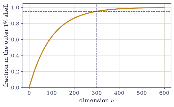
Fig. 431 Concentration of measure: a high-dimensional ball is almost all skin. The fraction of an \(n\)-ball’s volume lying in the outer \(1\%\) of its radius, \(1-(0.99)^n\), against dimension \(n\). By \(n=300\) (dashed) it is \(95\%\); by \(n=3000\) (a gas of a thousand particles) essentially all of the volume sits in a vanishingly thin shell at the surface. This is why the microcanonical entropy does not depend on the shell thickness \(\Delta E\) — the ball and the shell are the same thing in high dimensions — and it is the geometric face of the \(1/\sqrt N\) sharpening of §5.3.#
Exercise 3 — Entropy and the caloric equation of state (worked)#
Now the payoff begins. With the multiplicity in hand, entropy is \(S=k\ln\Omega\) (§5.4), and temperature is the energy-slope \(1/T=\partial S/\partial E\) — the definition we earned in §5.4, applied now to the continuous gas. Because \(\Sigma\propto E^{3N/2}\), that derivative is immediate: \(\partial(\ln\Sigma)/\partial E=3N/2E\), so \(1/T=3N/2E\), which rearranges to the caloric equation of state \(E=\tfrac32 NkT\) Eq. 412. This is equipartition, exact and from first principles: each of the \(3N\) translational degrees of freedom carries \(\tfrac12 kT\) of energy. The same statement we will keep meeting — every quadratic degree of freedom gets \(\tfrac12 kT\) — here falls straight out of the geometry of a high-dimensional ball.
Part a) Tabulate the entropy \(S/k=\ln\Sigma\) on a grid of \(201\) energies spanning \(0.7E_0\) to
\(1.3E_0\), with the ln_Sigma you wrote in Exercise 1, and differentiate it with numpy.gradient
to obtain \(1/T=\partial S/\partial E\) at every energy.
Part b) Read off \(T\) at the working energy \(E_0\) and confirm the caloric equation of state \(E=\tfrac32 NkT\) — equipartition, \(\tfrac12 kT\) for each of the \(3N\) translational degrees of freedom.
1/T = ∂S/∂E at E=1500.0:  T = 1.00000
caloric equation of state: E = 1500.0   vs   (3/2)NkT = 1499.995
→ equipartition: each of the 3N=3000 translational dof carries ½kT
Validation 3#
✓ 1/T = ∂S/∂E gives the caloric equation of state E = (3/2)NkT (equipartition) [got 1500 vs expected 1500 (rtol=0.001, atol=1e-09)]
True
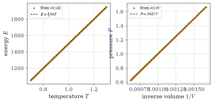
Fig. 432 The two equations of state, read off the entropy. Left: energy versus temperature, \(T\) obtained as \((\partial S/\partial E)^{-1}\) across a grid of energies; the points fall on the line \(E=\tfrac32 NkT\) (dashed) — the caloric equation of state, i.e. equipartition for \(3N\) translational degrees of freedom. Right: pressure versus inverse volume, \(P=T\,\partial S/\partial V\); the points fall on \(P=NkT/V\) (dashed) — the ideal gas law, derived here from the phase-space volume rather than assumed. Both equations of state are derivatives of one entropy.#
Exercise 4 — Pressure and the ideal gas law (worked)#
The second derivative gives the second equation of state, and it is one of the most famous results in physics — obtained here without ever assuming it. Pressure enters thermodynamics as the volume-slope of entropy, \(P/T=\partial S/\partial V\) Eq. 412. From \(\ln\Sigma\) the only \(V\)-dependence is the positional factor \(N\ln V\), so \(\partial S/\partial V=N/V\), giving \(P/T=N/V\), that is \(PV=NkT\) — the ideal gas law (Fig. 432, right). Boyle, Charles, and Gay-Lussac measured this over centuries; here it drops out of the geometry of phase space in one line. That is the power of the microcanonical method: the macroscopic equation of state is a derivative of a counted (here, integrated) multiplicity.
Part a) Compute the pressure \(P=T\,\partial S/\partial V\) at the working state, as a central
difference of the Exercise 1 ln_Sigma in the volume, at the temperature \(T\) of Exercise 3.
Part b) Confirm the thermal equation of state \(PV=NkT\), and read the ideal gas law off the volume sweep in Fig. 432 (right).
P/T = ∂S/∂V at V=1000.0:  P = 1.00000
thermal equation of state: PV = 999.997   vs   NkT = 999.997
Validation 4#
✓ P/T = ∂S/∂V gives the thermal equation of state PV = NkT (the ideal gas law) [got 999.997 vs expected 999.997 (rtol=0.001, atol=1e-09)]
True
Exercise 5 — The chemical potential (worked)#
The third derivative names a quantity we have not met but will lean on heavily: the chemical potential \(\mu=-T\,\partial S/\partial N\) Eq. 413, the change in energy when one particle is added at fixed entropy and volume — equivalently, how much entropy a new particle brings. For a dilute classical gas \(\mu\) is negative: adding a particle at fixed total energy and volume raises the entropy (there are more ways to arrange more particles), so \(-T\,\partial S/\partial N<0\). The chemical potential is the quantity that equalizes when particles are free to flow — across a membrane, between phases, in a chemical reaction — exactly as temperature equalizes for energy flow. It is the star of the grand canonical ensemble later in the volume, and the link from statistical mechanics to chemistry.
There is a closed form to check against: applying Stirling’s approximation to the \(N!\) and the \(\Gamma(\tfrac{3N}{2}+1)\) in \(\ln\Sigma\) and differentiating gives \(\mu=-kT\ln\!\big[(V/N)(2\pi mkT)^{3/2}/h^3\big]\) for the ideal gas, the logarithm of the number of thermal wavelengths per particle.
Part a) Compute \(\partial S/\partial N\) as a finite difference of the Exercise 1 ln_Sigma in
the integer \(N\) (evaluate at \(N\pm1\)), form \(\mu=-T\,\partial S/\partial N\) with the Exercise 3
temperature, and confirm it comes out negative for the dilute classical gas.
Part b) Evaluate the Stirling closed form above in the notebook’s units and confirm the two routes to \(\mu\) agree.
∂S/∂N = 2.7558  (adding a particle raises the entropy)
chemical potential μ = −T ∂S/∂N = -2.7558   (negative for the dilute classical gas)
closed form −kT ln[(V/N)(2πmkT)^(3/2)/h³] = -2.7568  (agree)
μ is the energy cost of a particle — the quantity that equalizes when particles can flow
Validation 5#
✓  μ = −T ∂S/∂N matches the closed form −kT ln[(V/N)(2πmkT)^(3/2)/h³]   [got -2.75581 vs expected -2.7568 (rtol=0.01, atol=1e-09)]
✓  the dilute classical gas has a negative chemical potential
True
Exercise 6 — The fundamental thermodynamic relation (worked)#
Now we collect the three derivatives into a single statement that is, arguably, the master equation of equilibrium thermodynamics. If \(S\) is a function of \(E\), \(V\), and \(N\), then any small change in energy decomposes as \(dU=T\,dS-P\,dV+\mu\,dN\) Eq. 414 — equivalently \(dS=\tfrac1T dU+\tfrac PT dV-\tfrac{\mu}{T}dN\), which is just the chain rule with our three slopes \(\partial S/\partial E=1/T\), \(\partial S/\partial V=P/T\), \(\partial S/\partial N=-\mu/T\). This one differential packages the first law (energy bookkeeping) and the second (entropy as the state function whose slopes are \(T,P,\mu\)). Everything in §5.7 — the thermodynamic potentials, the Legendre transforms that swap which variables are held fixed, the Maxwell relations — is built on this relation. We can check it is no mere tautology by verifying it numerically: take a small, simultaneous step in \((E,V,N)\) and confirm the directly computed entropy change matches the one the relation predicts from the three slopes.
Part a) For a small simultaneous step \((dE,dV,dN)=(15,10,2)\), compute the entropy change
directly, as the difference of the Exercise 1 ln_Sigma between the stepped state and the
working state.
Part b) Assemble the same change from the three slopes as \(\tfrac1T dU+\tfrac PT dV-\tfrac{\mu}{T}dN\), using the \(T\), \(P\) and \(\mu\) of Exercises 3, 4 and 5, and confirm the two agree — the fundamental relation is a numerical identity, not a definition.
step (dE,dV,dN) = (15.0, 10.0, 2)
dS direct (from ln Σ)              = 30.4322
dS from (1/T)dU+(P/T)dV−(μ/T)dN    = 30.5117
agreement: 0.26%  → the fundamental relation holds
Validation 6#
✓ the fundamental relation dU = TdS − PdV + μdN holds for the ideal gas [got 30.4322 vs expected 30.5117 (rtol=0.02, atol=1e-09)]
True
Exercise 7 — Maxwell–Boltzmann as the shadow of the sphere (worked)#
We turn from thermodynamics to the velocities themselves, and find the first statistical law ever written in physics hiding in the geometry of a sphere. Fix the total kinetic energy: then the \(3N\) velocity components satisfy \(\sum\tfrac12 m v_i^2=E\), so the velocity vector lives uniformly on a sphere of radius \(R=\sqrt{2E/m}\) in \(3N\) dimensions (the microcanonical measure for free particles). What does one component look like? It is the shadow of that uniform sphere cast on a single axis. For \(n=3\) this shadow is exactly uniform (Archimedes’ hat-box theorem); but as \(n\) grows the shadow becomes a Gaussian (Fig. 434), by the same central-limit mechanism as §5.3 — the variance of one coordinate of a uniform \(n\)-sphere point is \(R^2/n=kT/m\) Eq. 415. That Gaussian is the Maxwell–Boltzmann velocity distribution (Maxwell, 1860), and this is its deepest explanation: the famous factor \(e^{-mv^2/2kT}\) is the projection of a high-dimensional energy sphere. The speed of one particle then follows \(f(v)\propto v^2 e^{-mv^2/2kT}\), with \(\langle v\rangle=\sqrt{8kT/\pi m}\) and \(v_{\rm rms}=\sqrt{3kT/m}\) (Fig. 433).
To see the shadow we must first draw the sphere, and there is a trick for that. A vector of
independent standard Gaussians has a distribution that depends only on its length — it has no
preferred direction — so rescaling it to a fixed length \(R\) lands it uniformly on the sphere of
radius \(R\), in any number of dimensions. That is the only honest way to sample a \(3000\)-sphere,
and it is one line of numpy.linalg.norm once seen.
Part a) Write sample_velocity_sphere(N, E, m, n_samples, rng), returning n_samples
velocity vectors drawn uniformly from the constant-energy sphere of radius \(R=\sqrt{2E/m}\) in
\(3N\) dimensions: draw an (n_samples, 3N) block of standard Gaussians from rng and rescale each
row to length \(R\). Write this one yourself — the implementation is the lesson.
Part b) Draw \(6000\) samples for the working state and confirm that a single velocity component is Gaussian with variance \(kT/m\) — Maxwell–Boltzmann as the projection of the energy sphere.
Part c) Form the speed of one particle from its three components and confirm the Maxwell–Boltzmann \(\langle v\rangle=\sqrt{8kT/\pi m}\) and \(v_{\rm rms}=\sqrt{3kT/m}\).
The animation that follows shows the single-component shadow morphing from uniform (\(n=3\)) to Gaussian as the dimension grows — concentration of measure building the Boltzmann factor before our eyes.
one velocity component: variance = 0.9910  vs  kT/m = 1.0000
speed ⟨v⟩   = 1.5835  vs  √(8kT/πm) = 1.5958
speed v_rms = 1.7201  vs  √(3kT/m)  = 1.7320
Validation 7#
✓  one velocity component is Gaussian with variance kT/m — Maxwell–Boltzmann as the projection of the energy sphere   [got 0.991024 vs expected 0.999997 (rtol=0.03, atol=1e-09)]
✓  the speed obeys the Maxwell–Boltzmann law   [max|Δ| = 0.012272 (rtol=0.03, atol=1e-09)]
True
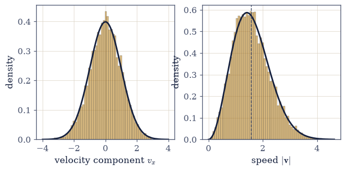
Fig. 433 The Maxwell–Boltzmann distribution, sampled from the energy sphere. Left: the histogram of a single velocity component (amber) against the Gaussian \(\mathcal N(0,kT/m)\) (dark) — the shadow of the \(3N\)-sphere on one axis. Right: the speed of one particle (amber) against the Maxwell–Boltzmann law \(f(v)\propto v^2 e^{-mv^2/2kT}\) (dark), with \(\langle v\rangle=\sqrt{8kT/\pi m}\). Maxwell wrote this in 1860, the first statistical law in physics; here it is a geometric fact about high-dimensional spheres, and the factor \(e^{-mv^2/2kT}\) is revealed as a projection.#
Fig. 434 Why the shadow is Gaussian (animated). The marginal of one component of a uniform point on an \(n\)-sphere (rescaled to unit variance), as the dimension \(n\) grows. At \(n=3\) it is flat — Archimedes’ theorem: the projection of a uniform sphere onto an axis is exactly uniform. As \(n\) increases the distribution rounds into the standard Gaussian (dark), reached well before \(n=100\). This is concentration of measure / the central limit theorem of §5.3 in action, and it is precisely the mechanism that turns the fixed-energy velocity sphere into the Maxwell–Boltzmann distribution.#
Exercise 8 — The Gibbs paradox and the limit of classical counting (worked)#
Here, at last, classical mechanics genuinely fails — and the way it fails is one of the most instructive moments in the subject. Take two boxes of the same gas, each \((N,V,E)\), and remove the wall. Physically nothing happens: it is the same gas at the same temperature and pressure, so the entropy should not change. But if we use the naive multiplicity without the \(1/N!\), the computed entropy jumps by a spurious \(2Nk\ln 2\) Eq. 416 — the Gibbs paradox (Fig. 435). Including the \(1/N!\), which treats the particles as indistinguishable, restores extensivity and the jump vanishes (up to an \(O(\ln N)\) finite-size remnant that the thermodynamic limit removes). Yet here is the honest catch: why \(1/N!\), and the value of \(h\) that fixes the absolute entropy (the Sackur–Tetrode equation \(S=Nk[\ln(V/N\lambda^3)+\tfrac52]\) with \(\lambda=h/\sqrt{2\pi mkT}\)), are both quantum in origin. Classical mechanics gives the form of the entropy and every difference correctly, but cannot justify the indistinguishability factor or set the absolute scale on its own. We state Sackur–Tetrode, attribute its \(\hbar\) and \(1/N!\) to quantum mechanics, and defer the derivation to Volume VII — classical physics taken exactly as far as it honestly goes, the same move as Mercury’s perihelion. And to be clear the paradox is about identical gases: mixing two different gases really does raise the entropy by \(2Nk\ln 2\), the physical entropy of mixing \(-k\sum x\ln x\) of §5.3.
The gibbs switch you built into ln_Sigma in Exercise 1 is what makes the comparison possible:
the same function, with and without the \(1/N!\), on two boxes of \((N,V,E)=(600,600,900)\) — a state
at the same \(T=1\) — combined into one \((2N,2V,2E)\).
Part a) Compute the entropy change on combining the two identical boxes without the Gibbs factor, and confirm it is the spurious \(2Nk\ln2\): a number where physically nothing happened.
Part b) Repeat with the Gibbs factor and confirm the change per particle is \(\approx0\) — extensivity restored, up to the \(O(\ln N)\) finite-size remnant.
Part c) Now let the two gases be different: each species expands from \(V\) into \(2V\) at fixed energy, keeping its own \(\ln\Sigma\). Confirm this change is the real \(2Nk\ln2\) — the same number, spurious in Part a and physical here.
combine two identical (600,600.0,900.0) boxes → (2N,2V,2E):
  WITHOUT 1/N!:  ΔS = 835.8   (spurious — the Gibbs paradox; ≈ 2N ln2 = 831.8)
  WITH    1/N!:  ΔS = 7.74   (≈ 0 per particle: 0.0129/particle — extensive, up to O(ln N))

different gases mixing: ΔS = 2Nk ln2 = 831.8  (real — the §5.3 entropy of mixing)
Validation 8#
✓  without the Gibbs 1/N! the entropy gains a spurious 2Nk ln2 on combining identical gases (the Gibbs paradox)   [got 835.75 vs expected 831.777 (rtol=0.02, atol=1e-09)]
✓  the Gibbs 1/N! restores extensivity — combining identical gases changes the entropy per particle by ≈0   [got 0.0129079 vs expected 0 (rtol=1e-06, atol=0.02)]
✓  mixing DIFFERENT gases gives the real entropy of mixing 2Nk ln2   [got 831.777 vs expected 831.777 (rtol=1e-12, atol=1e-09)]
True
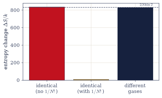
Fig. 435 The Gibbs paradox. Entropy change on combining two boxes of gas. Left two bars: two identical boxes merged — without the \(1/N!\) the entropy jumps by a spurious \(2Nk\ln2\) (nothing physical happened), while with the indistinguishability factor it is \(\approx0\), as it must be. Right bar: two different gases mixed — a real \(2Nk\ln2\), the physical entropy of mixing. The same number is spurious in one case and real in the other; the resolution, indistinguishability, is quantum in origin and is the honest cliffhanger to Volume VII.#
Exercise 9 — Equipartition beyond translation, and the route to real gases (student)#
Before the synthesis, one extension that both broadens equipartition and plants a flag for what classical mechanics cannot do. Our \(E=\tfrac32 NkT\) counted \(3N\) translational degrees of freedom, each quadratic in a momentum, each carrying \(\tfrac12 kT\). But equipartition counts any quadratic degree of freedom — and a diatomic molecule can also rotate, adding two rotational quadratic terms. So a classical diatomic gas has \(5\) quadratic degrees of freedom per molecule and a heat capacity \(C_V=\tfrac52 Nk\) Eq. 412 (and a rigid polyatomic, \(3\) rotations, gives \(3Nk\)). This is the classical prediction — and it is wrong at low temperature, where measured heat capacities fall below it as the rotational and vibrational modes “freeze out.” That freezing is quantum: the modes have discrete energy gaps that \(kT\) cannot bridge when it is small, another question deferred to Volume VII. (And for interacting gases the position integral no longer factorizes into \(V^N\) — the configurational integral with \(U(r)\) is the route to the virial expansion and the van der Waals equation, the foundational next step beyond the ideal gas.)
Part a) Measure the translational heat capacity from the microcanonical \(T(E)\) of Exercise 3:
\(C_V=dE/dT\) with numpy.gradient on that same grid, read at the working energy. It must come out
\(\tfrac32 Nk\) — \(\tfrac12 k\) per quadratic degree of freedom, measured rather than assumed.
Part b) Add the \(2\) rotational quadratic degrees of freedom of a diatomic molecule and confirm the classical \(C_V=\tfrac52 Nk\) — a prediction whose low-temperature failure, the freeze-out of rotation and vibration, is quantum and waits for Volume VII.
diatomic gas: 3 translational + 2 rotational quadratic dof
measured translational C_V = dE/dT = 1500.0  vs  (3/2)Nk = 1500.0
C_V = ½(3+2)Nk = 2500.0  vs  (5/2)Nk = 2500.0
classical prediction — the freezing-out of rotation/vibration at low T is quantum (Volume VII)
Validation 9#
✓  the measured microcanonical heat capacity is (3/2)Nk — ½k per quadratic degree of freedom   [got 1500 vs expected 1500 (rtol=0.01, atol=1e-09)]
✓  adding the two rotational degrees of freedom gives the diatomic C_V = (5/2)Nk   [got 2500 vs expected 2500 (rtol=1e-12, atol=1e-09)]
True
Exercise 10 — All of thermodynamics from a phase-space volume (synthesis)#
Look back at what one integral bought. From the volume of the energy shell — an honest ball in \(3N\) dimensions, regulated by a \(\Gamma\) function and computed in log space because it overflows — we obtained the entropy \(S=k\ln\Sigma\). Its three derivatives gave the entire equilibrium thermodynamics of the gas: the caloric equation of state \(E=\tfrac32NkT\), the thermal one \(PV=NkT\), the chemical potential \(\mu=-T\,\partial S/\partial N\), and the fundamental relation \(dU=T\,dS-P\,dV+\mu\,dN\) that packages them. Concentration of measure assured us the shell and the ball agree; the Maxwell–Boltzmann velocity law turned out to be the shadow of the energy sphere, a Gaussian by the central-limit mechanism of §5.3; and the one genuine failure — the absolute entropy and the Gibbs \(1/N!\) — became an honest deferral to the quantum volume. We bore the full cost of doing statistical mechanics classically: a \(6N\)-dimensional integral rather than a binomial coefficient. The next notebook (§5.7) takes the fundamental relation and builds the thermodynamic potentials and Maxwell relations on it, with the Legendre transform of Volume II as the key.
There is nothing left to compute: the argument is the result. We computed one high-dimensional volume and differentiated it three ways, and out came an entire science. That a macroscopic equation of state is a derivative of a microscopic phase-space volume is the whole idea of statistical mechanics, and the ideal gas is where it is seen most cleanly.
Notebook summary#
From the phase-space volume of a classical gas, all of equilibrium thermodynamics followed by differentiation — the heavier classical machinery developed in full, because the integral is the physics.
The phase-space volume Eq. 410: \(\Sigma=V^N\pi^{3N/2}(2mE)^{3N/2}/(\Gamma(\tfrac{3N}{2}+1)h^{3N}N!)\), computed as \(\ln\Sigma\) with
scipy.special.gammalnbecause it overflows (§5.3/§0.1, in \(3N\) dim).Concentration of measure Eq. 411: \(1-(1-\varepsilon)^n\to1\) (the outer \(1\%\) of a \(300\)-ball holds \(95\%\)); the shell and ball give the same temperature to \(O(1/N)\).
The equations of state Eq. 412: \(1/T=\partial S/\partial E\Rightarrow E=\tfrac32NkT\) (equipartition) and \(P/T=\partial S/\partial V\Rightarrow PV=NkT\) (the ideal gas law, derived).
The chemical potential Eq. 413: \(\mu=-T\,\partial S/\partial N\approx-2.76\) (negative for the dilute gas), the quantity that governs particle exchange.
The fundamental relation Eq. 414: \(dU=T\,dS-P\,dV+\mu\,dN\), verified as a numerical identity — the master equation §5.7 builds the potentials on.
Maxwell–Boltzmann Eq. 415: one velocity component is the Gaussian shadow of the energy sphere (\(\operatorname{Var}=kT/m\)), uniform at \(n=3\) and Gaussian as \(n\) grows; the speed law gives \(\langle v\rangle=\sqrt{8kT/\pi m}\), \(v_{\rm rms}=\sqrt{3kT/m}\).
The Gibbs paradox Eq. 416: \(1/N!\) restores extensivity (spurious \(2Nk\ln2\to0\)); its quantum origin, and the absolute Sackur–Tetrode entropy, are deferred to Volume VII. Mixing different gases gives the real \(2Nk\ln2\).
We bought the whole of equilibrium thermodynamics with one \(6N\)-dimensional integral.
Outlook#
Thermodynamic potentials and Maxwell relations (§5.7). Take the fundamental relation and build the free energies by Legendre transform (the Volume II transform again), with the Maxwell relations as the integrability conditions — the working machinery of thermodynamics.
The chemical potential and the grand canonical ensemble. \(\mu\) comes into its own when particle number can fluctuate — the ensemble for open systems, later in the volume.
Real gases. The configurational integral with interactions \(U(r)\) no longer factorizes into \(V^N\): the route to the virial expansion and the van der Waals equation, the foundational step beyond the ideal gas.
Quantum statistics (Volume VII). The Sackur–Tetrode entropy derived, the \(1/N!\) and \(h\) justified by indistinguishability, and the quantum gases (Fermi–Dirac, Bose–Einstein) where the freeze-out of internal modes and degeneracy take over.
Cross-reference §5.4 (microcanonical entropy and \(1/T=\partial S/\partial E\)), §5.3 (large-\(N\), the Gaussian/CLT, the entropy of mixing), §0.1 (log space).