


3.11 RLC and AC Circuits#
Notebook overview#
This notebook is a homecoming. The series RLC circuit, a resistor, inductor, and capacitor driven by an oscillating source, obeys the equation \(L\ddot q+R\dot q+q/C= V(t)\), and that is, term for term, the damped driven oscillator \(m\ddot x+b\dot x+kx= F(t)\) we already solved in §1.2. Inductance plays the part of mass, resistance of friction, and the inverse capacitance \(1/C\) of the spring constant. Everything that took work to understand in mechanics, natural frequency, damping regimes, resonance, the quality factor \(Q\), the phase lag, the exchange of energy, transfers wholesale. We have solved this circuit before, in mechanics, and the point of the notebook is to feel that.
We build the equation from Kirchhoff’s voltage law, using the inductor relation from Faraday’s induction (§3.7) and the capacitor relation from electrostatics (§3.2), then lay it beside the mechanical oscillator and integrate both to watch them coincide to machine precision. We meet the complex impedance \(Z=R+i(\omega L-1/\omega C)\), the bookkeeping trick that turns differential equations into algebra, find the resonance where the reactances cancel and the current peaks, compute the quality factor three equivalent ways, draw the phasor diagram that makes the phase relationships visible, and watch energy slosh between the inductor and capacitor exactly as kinetic and potential energy trade in a mass on a spring. The generator of §3.7 finally drives the circuit it was built for, closing a loop in the volume.
Everything is in SI units. The circuit’s transient ring-down is genuine temporal
evolution, so exactly one figure is animated, the energy oscillating between \(L\) and
\(C\); everything else is a still. Circuit diagrams follow the international IEC 60617
standard (a rectangle resistor, not the American zigzag), drawn with the shared
ecp.draw circuit primitives.
How to read the checks. Each exercise ends with a
validatecall against an independent fact: the RLC charge equal to the mechanical displacement, the natural frequency \(1/\sqrt{LC}\), the impedance equal to \(R\) at resonance, the three forms of \(Q\) agreeing, the average power \(\tfrac12 V_0 I_0\cos\varphi\). A ✓ is strong evidence; a ✗ is a prompt to locate the discrepancy, not a verdict.Scope. A working review, not a full circuits course. See Nolting, Theoretical Physics 3 [Nol16]; Griffiths, Introduction to Electrodynamics [Gri17]; and §1.2 throughout, of which this is the electrical twin.
Theory in brief#
The circuit equation from Kirchhoff#
Summing the voltage drops around a series loop, across the inductor (\(L\,dI/dt\), from Faraday’s law, §3.7), the resistor (\(RI\)), and the capacitor (\(q/C\), from §3.2), and setting them equal to the source gives
The mechanical correspondence (the spine)#
Equation Eq. 249 is term-by-term the damped driven oscillator \(m\ddot x+b\dot x+ kx=F(t)\) of §1.2, under the dictionary
So the natural frequency is \(\omega_0=1/\sqrt{LC}\) (the analogue of \(\sqrt{k/m}\)) and the damping rate \(\gamma=R/2L\) (the analogue of \(b/2m\)); the under-, critically, and over-damped regimes carry across unchanged.
Transient response#
With the source off, the homogeneous solution Eq. 249 is the ring-down: an underdamped circuit oscillates at \(\approx\omega_0\) with an envelope \(e^{-\gamma t}\), the exact electrical image of the mechanical transient of §1.2 and §1.6.
AC steady state and complex impedance#
For \(V(t)=V_0\cos\omega t\) the steady-state current is most easily found with the complex impedance. Writing every sinusoid as the real part of a complex exponential \(\propto e^{i\omega t}\) turns each time derivative in Eq. 249 into a factor of \(i\omega\), so Kirchhoff’s sum becomes ordinary algebra with
built from \(Z_R=R\), \(Z_L=i\omega L\), \(Z_C=1/i\omega C\). The differential equation becomes algebra.
Resonance and the quality factor#
The current resonates at \(\omega_0\), where the reactances cancel (\(\omega L=1/\omega C\)), \(|Z|\) is minimal and equal to \(R\), and the current is maximal and in phase with the source. The sharpness is the quality factor
the same \(Q\) as the mechanical oscillator, setting both the resonance width (\(\approx\omega_0/Q\)) and the ring-down rate.
Phasors and energy#
Representing each sinusoid as a rotating vector (a phasor), the voltage across \(R\) is in phase with the current, \(V_L\) leads by \(90°\), and \(V_C\) lags by \(90°\); their vector sum is the source voltage,
Energy oscillates between the inductor (\(\tfrac12 LI^2\), the “kinetic” store) and the capacitor (\(\tfrac12 q^2/C\), the “potential” store), dissipated by \(R\),
exactly the kinetic–potential exchange with friction of the mechanical oscillator.
Setup#
Data only, in SI units: the running series-RLC values (\(L=1\,\)mH, \(R=10\,\Omega\), \(C=1\,\mu\)F, \(V_0=5\,\)V, chosen so that \(Q=\sqrt{10}\)), the natural frequency \(\omega_0=1/\sqrt{LC}\) that follows from them, the series palette, and two formulas the theory above hands over outright — the complex impedance \(Z(\omega)\) Eq. 251 and the three closed forms of the quality factor Eq. 252. Each of those is a one-line transcription of a displayed equation with nothing to construct, so neither is anyone’s lesson here.
The circuit’s equations of motion are deliberately absent: you write the RLC and the mechanical state derivatives yourself in Exercise 1, and every integration in the notebook — the ring-down, the energy exchange, the generator drive — runs on the ones you wrote. No randomness appears anywhere in this notebook.
The Setup below holds this notebook’s data and instruments — nothing you are asked to build. It is collapsed so the building stays yours; expand it whenever you want the details.
Exercise 1 — The RLC equation and the mechanical mirror (worked)#
Kirchhoff’s voltage law around the series loop sums the drops across the inductor (\(L\,dI/dt\)), resistor (\(RI\)), and capacitor (\(q/C\)) to the source, giving \(L\ddot q+ R\dot q+q/C=V(t)\) Eq. 249 (Fig. 278). Set it beside the damped driven oscillator of §1.2 and the two are the same equation under \(L\leftrightarrow m\), \(R\leftrightarrow b\), \(1/C\leftrightarrow k\) Eq. 250. We are not learning a new problem; we are re-reading an old one.
An adaptive solver wants a first-order system, so each second-order equation has to be recast in a two-component state — \([q,I]\) with \(I=\dot q\) for the circuit, \([x,v]\) with \(v=\dot x\) for the mass — whose derivative is \([\,I,\ (V-RI-q/C)/L\,]\) and \([\,v,\ (F-bv-kx)/m\,]\) respectively. Written out, those two lines are the same line. The circuit values are \(L=1\,\)mH, \(R=10\,\Omega\), \(C=1\,\mu\)F and \(V_0=5\,\)V, the drive sits at \(0.7\,\omega_0\), and both systems start from rest. The two curves must then coincide to solver precision: we are solving §1.2 again, in electrical clothing.
Write
rlc_rhs(t, y, L, R, C, drive)andosc_rhs(t, y, m, b, k, drive), the state derivatives of the circuit Eq. 249 and of the mechanical oscillator, each returning the two-element list above for ascipy.integrate.solve_ivpcall. Keep them as separate functions even though the bodies match — that duplication is the point. Write these yourself — the implementation is the lesson, and every integration in this notebook runs onrlc_rhs.Integrate the RLC charge \(q(t)\) with
scipy.integrate.solve_ivp(DOP853).Separately integrate the mechanical \(x(t)\) with \(m=L\), \(b=R\), \(k=1/C\), and compare the two curves.
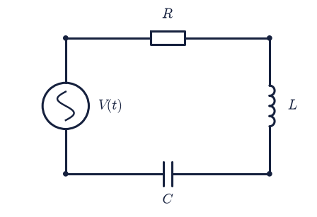
Fig. 278 The series RLC circuit (IEC 60617 symbols): an AC source \(V(t)\), a resistor \(R\) (a plain rectangle), an inductor \(L\) (a coil), and a capacitor \(C\) (parallel plates), in a single loop. Kirchhoff’s voltage law around the loop gives \(L\ddot q+R\dot q+q/C=V(t)\), term-for-term the damped driven oscillator of §1.2 with \(L\leftrightarrow m\), \(R\leftrightarrow b\), \(1/C\leftrightarrow k\).#
ω₀ = 1/√(LC) = 31622.8 rad/s  (f₀ = 5032.9 Hz)
max |q_RLC(t) − x_mech(t)| = 4.86e-15
Validation 1#
✓ the RLC charge and the mechanical displacement are the same function (L↔m, R↔b, 1/C↔k) [max|Δ| = 4.85867e-15 (rtol=1e-09, atol=1e-13)]
True
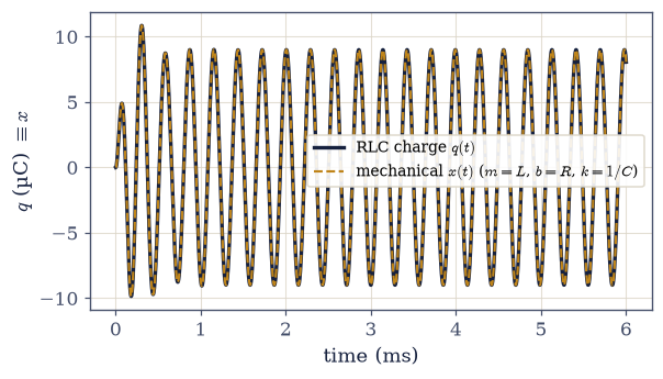
Fig. 279 The RLC charge \(q(t)\) (dark) and the mechanical displacement \(x(t)\) (amber dashed) for the driven systems, plotted together. They lie exactly on top of one another: the two curves differ by less than \(10^{-14}\) over the whole run, because \(L\ddot q+R\dot q+q/C=V\) and \(m\ddot x+b\dot x+kx=F\) are literally the same differential equation. The RLC circuit is the mechanical oscillator of §1.2 in electrical clothing.#
Exercise 2 — Natural frequency and damping regimes (worked)#
Switch the source off, charge the capacitor, and release: the circuit rings down, just as a plucked mass-spring does. The natural frequency is \(\omega_0=1/\sqrt{LC}\) and the damping rate \(\gamma=R/2L\), and the comparison of the two sorts the behaviour into the same three regimes as §1.2: underdamped (\(\gamma<\omega_0\), oscillatory decay), critically damped (\(\gamma=\omega_0\), fastest non-oscillatory return), and overdamped (\(\gamma>\omega_0\), sluggish return). The boundary sits at the critical resistance \(R=2\sqrt{L/C}\), where \(\gamma=\omega_0\) exactly.
Confirm that the running circuit’s natural frequency is \(\omega_0=1/\sqrt{LC}\).
Integrate the source-free circuit (\(C\) initially charged, drive switched off) with the
rlc_rhsyou wrote in Exercise 1, for three resistances spanning the regimes, and watch the ring-down change character (Fig. 280) — the electrical echo of the mechanical damping regimes.
ω₀ = 31622.8 rad/s,  critical R = 2√(L/C) = 63.25 Ω
γ = R/2L:  under 5000.0 < ω₀ 31622.8 = crit 31622.8 < over 300000.0
Validation 2#
✓  the natural frequency is 1/√(LC)   [got 31622.8 vs expected 31622.8 (rtol=1e-09, atol=1e-09)]
✓  the damping regimes follow from γ = R/2L versus ω₀: γ_under < ω₀ = γ_crit < γ_over
True
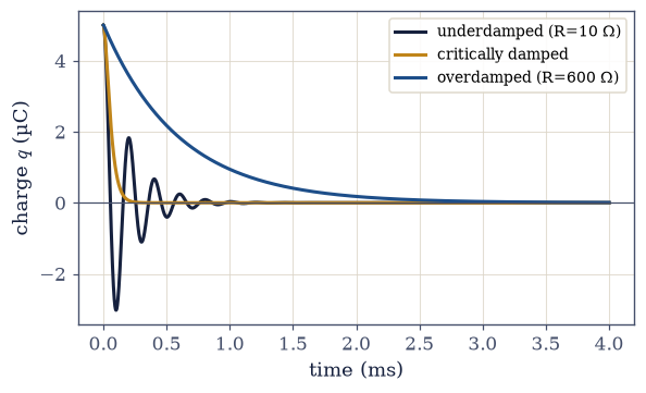
Fig. 280 Source-free ring-down of the charge \(q(t)\) from an initially charged capacitor, for three resistances. Underdamped (\(R=10\,\Omega\), \(\gamma<\omega_0\)): oscillatory decay at \(\approx\omega_0\). Critically damped (\(R=2\sqrt{L/C}\)): the fastest return with no overshoot. Overdamped (\(R=600\,\Omega\), \(\gamma>\omega_0\)): a slow crawl back to zero. These are exactly the damping regimes of the mechanical oscillator of §1.2.#
Exercise 3 — Energy exchange between L and C (worked)#
In an underdamped ring-down the total energy does not just decay; it sloshes. Energy pours from the capacitor (electric, \(\tfrac12 q^2/C\), the “potential” store) into the inductor (magnetic, \(\tfrac12 LI^2\), the “kinetic” store) and back, twice per cycle, while the resistor bleeds the total away Eq. 254. This is precisely the kinetic–potential exchange of a damped mass-spring, where energy trades between \(\tfrac12 mv^2\) and \(\tfrac12 kx^2\). A passive circuit can only lose energy, so the total \(E_L+E_C\) must fall monotonically, and the animation (Fig. 281) shows the two reservoirs filling and emptying in antiphase as it ebbs away.
For the underdamped ring-down (the
rlc_rhsyou wrote in Exercise 1, \(R=10\,\Omega\)), compute \(E_L(t)=\tfrac12 LI^2\) and \(E_C(t)=\tfrac12 q^2/C\).Confirm the two exchange — anti-correlated, \(180°\) out of phase, the fraction held in \(L\) swinging almost the whole way from \(0\) to \(1\) — while their sum decreases monotonically through \(R\).
energy fraction in L swings 0.00 → 1.00  (fully sloshes: True)
total energy monotonically decreasing: True
initial energy = 12.500 µJ,  final = 0.0000 µJ
Validation 3#
✓ energy oscillates between L and C (the fraction swings ≈0↔1) and decays through R
True
Fig. 281 Animation of the energy exchange in the underdamped ring-down. The inductor (magnetic, \(\tfrac12 LI^2\)) and capacitor (electric, \(\tfrac12 q^2/C\)) reservoirs fill and empty in alternation, \(180°\) out of phase, while the total (dark line) decays as the resistor dissipates it. This is the electrical image of kinetic and potential energy trading in a damped mass on a spring.#
Exercise 4 — Complex impedance (worked)#
Driven at a single frequency, the circuit is handled most cleanly with the complex impedance Eq. 251 \(Z(\omega)=R+i(\omega L-1/\omega C)\), which packages the resistor (\(R\)), inductor (\(i\omega L\)), and capacitor (\(1/i\omega C\)) into one complex number. The current amplitude is \(V_0/|Z|\) and its phase lag is \(\arg Z\); the differential equation has become algebra. At \(\omega_0\) the inductive and capacitive reactances cancel exactly, so the imaginary part vanishes and \(|Z|=R\): the circuit looks purely resistive there, and that is why the current peaks.
Evaluate the Setup
impedanceover a frequency sweep from \(0.2\,\omega_0\) to \(3\,\omega_0\) and plot \(|Z|\) and \(\arg Z\) (Fig. 282).Confirm that at \(\omega_0\) the impedance is purely resistive, \(|Z|=R\), and that the residual reactance there is round-off rather than physics.
|Z(ω₀)| = 10.000000 Ω   (R = 10.000000 Ω)
reactance at ω₀: ωL − 1/ωC = -3.55e-15 Ω (cancels)
Validation 4#
✓ at resonance the impedance is purely resistive, |Z| = R [got 10 vs expected 10 (rtol=1e-06, atol=1e-09)]
True
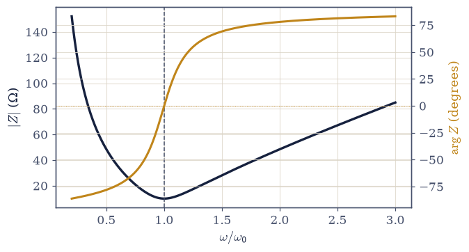
Fig. 282 Magnitude \(|Z|\) (dark) and phase \(\arg Z\) (amber) of the series impedance against frequency. \(|Z|\) dips to its minimum \(R\) at \(\omega_0\) (dashed), where the reactances cancel; below \(\omega_0\) the capacitor dominates and the phase is negative (capacitive), above it the inductor dominates and the phase is positive (inductive). The dip in \(|Z|\) is what makes the current peak at resonance.#
Exercise 5 — Resonance and the quality factor (worked)#
The current amplitude \(I_0(\omega)=V_0/|Z(\omega)|\) peaks where \(|Z|\) dips, at \(\omega_0\) Eq. 252. How sharp that peak is, and how slowly the circuit rings down, are one number: the quality factor \(Q\), which can be written three equivalent ways, \(\omega_0 L/R=1/\omega_0 RC=(1/R)\sqrt{L/C}\). A high-\(Q\) circuit (small \(R\)) resonates sharply and rings for many cycles; a low-\(Q\) one is broad and dead. It is the same \(Q\) that governed the mechanical resonance of §1.2. For the running values the three forms should all give \(Q=\sqrt{10}\approx3.162\), and the resonance width should come out near \(\omega_0/Q\).
Confirm that the three forms of \(Q\) agree, using the Setup
quality_factor.Show that the current amplitude \(V_0/|Z(\omega)|\) peaks at \(\omega_0\).
Compare the resonance curves of a sharp (high-\(Q\), \(R=10\,\Omega\)) and a broad (low-\(Q\), \(R=40\,\Omega\)) circuit (Fig. 283).
Q = ω₀L/R = 3.1623,  1/ω₀RC = 3.1623,  (1/R)√(L/C) = 3.1623
current peaks at ω/ω₀ = 0.9990  (resonance at ω₀)
Validation 5#
✓  the three forms of Q agree (ω₀L/R = 1/ω₀RC = (1/R)√(L/C))   [max|Δ| = 8.88178e-16 (rtol=1e-06, atol=1e-09)]
✓  the current resonates at ω₀   [got 31591.1 vs expected 31622.8 (rtol=0.01, atol=1e-09)]
True
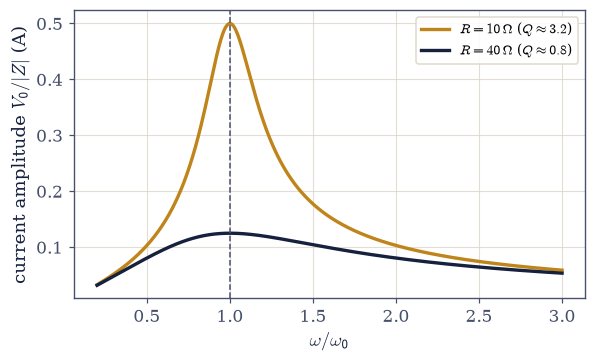
Fig. 283 Resonance curves: steady-state current amplitude \(V_0/|Z|\) against frequency, for a sharp high-\(Q\) circuit (\(R=10\,\Omega\), \(Q\approx3.2\), amber) and a broad low-\(Q\) one (\(R=40\,\Omega\), \(Q\approx0.8\), dark). Both peak at \(\omega_0\) (dashed), but the high-\(Q\) curve is tall and narrow, its full width at half maximum \(\approx\omega_0/Q\). This is the electrical twin of the mechanical resonance peak of §1.2.#
Exercise 6 — Phasors and phase (worked)#
A phasor turns each oscillating quantity into a rotating vector, and the algebra of sinusoids into vector addition Eq. 253. Taking the current as reference, the resistor voltage \(V_R=RI_0\) is in phase with it, the inductor voltage \(V_L=\omega L I_0\) leads by \(90°\), and the capacitor voltage \(V_C=I_0/\omega C\) lags by \(90°\); their vector sum is the source voltage. The angle between source and current is the phase lag \(\varphi=\arg Z\) (Fig. 284). Below \(\omega_0\) the capacitor wins, \(\arg Z<0\), and the current leads the source (the circuit is capacitive); above \(\omega_0\) the inductor wins and the current lags (inductive); at \(\omega_0\) the two are exactly in phase.
Compute \(\arg Z\) at \(0.5\,\omega_0\), at \(\omega_0\), and at \(2\,\omega_0\), and read off which way the current runs relative to the source in each case.
Draw the voltage phasors \(V_R\), \(V_L\), \(V_C\) and their sum at the frequency below resonance (Fig. 284).
below ω₀: arg Z = -78.1°  → current LEADS the source
at ω₀:    arg Z = -0.0°  → in phase
above ω₀: arg Z = +78.1°  → current LAGS the source
Validation 6#
✓  voltage and current are in phase at resonance (arg Z = 0)   [got -3.55271e-16 vs expected 0 (rtol=1e-06, atol=1e-06)]
✓  the current leads below ω₀ (capacitive) and lags above ω₀ (inductive)
True
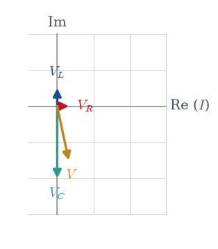
Fig. 284 Phasor diagram of the series RLC voltages at a drive below resonance, with the current along the real axis. \(V_R\) (red) is in phase with the current; \(V_L\) (blue) leads by \(90°\); \(V_C\) (green) lags by \(90°\). Their vector sum is the source voltage \(\mathbf V\) (amber). Below \(\omega_0\) the capacitor wins (\(V_C>V_L\)), so \(\mathbf V\) lies below the current: the current leads the source, the circuit is capacitive.#
Exercise 7 — The AC generator drives the circuit (student)#
In §3.7 a loop of \(N\) turns spun in a field produced the EMF \(\mathcal{E}=NBA\omega\sin \omega t\). That generator now drives the very circuit it was built for, completing a thread of the volume: §3.7 made the alternating EMF, and §3.11 uses it. The steady-state current it drives is set, as for any sinusoidal source, by the impedance, with amplitude \(\mathcal{E}_0/|Z(\omega)|\).
Build the generator EMF (state \(N\), \(B\), \(A\), \(\omega\)) and drive the RLC circuit with it, using the
rlc_rhsyou wrote in Exercise 1 throughscipy.integrate.solve_ivp(DOP853).Let the transient die away, and confirm the measured steady-state current amplitude matches the impedance prediction \(\mathcal{E}_0/|Z|\).
generator EMF amplitude NBAω = 8221.922 V
steady-state current: measured 420.8265 A  vs  ℰ₀/|Z| 420.8266 A
Validation 7#
✓ the generator drives a steady-state current set by the impedance, ℰ₀/|Z| [got 420.827 vs expected 420.827 (rtol=0.001, atol=1e-09)]
True
Exercise 8 — Average power and the power factor (student)#
Only the resistor consumes energy; the inductor and capacitor store it and hand it back. So the time-averaged power delivered by the source is \(\langle P\rangle=\tfrac12 V_0 I_0\cos\varphi\), where the power factor \(\cos\varphi\) measures how much of the current is in phase with the voltage. At resonance \(\varphi=0\), the power factor is one, and the delivery is maximal; far off resonance the current is mostly reactive and little power flows. Since the reactive elements give back everything they take, that average must equal \(\tfrac12 I_0^2 R\), the power dissipated in the resistor alone.
Drive the circuit at \(\omega=0.8\,\omega_0\) and integrate the instantaneous power \(V(t)\,I(t)\) over one full period with
numpy.trapezoid.Confirm the result equals \(\tfrac12 V_0 I_0\cos\varphi\), and equivalently \(\tfrac12 I_0^2 R\).
⟨P⟩ integrated  = 0.41322 W
½V₀I₀cosφ       = 0.41322 W   (power factor cosφ = 0.575)
½I₀²R (resistor) = 0.41322 W   (all power goes to R)
Validation 8#
✓ the average power is ½V₀I₀cosφ, delivered only to the resistor [got 0.413223 vs expected 0.413223 (rtol=0.001, atol=1e-09)]
True
Exercise 9 — One equation, two worlds#
Step back and see what the whole notebook rests on. A mass on a spring with friction and a charge in a circuit with resistance obey the same second-order linear differential equation. Resonance, damping, the quality factor, the phase lag, the exchange of energy between two stores: these are not analogies between two phenomena, they are one phenomenon wearing two costumes. That is why the computational tools built in mechanics, the integrators of §0.7, the resonance analysis of §1.2, the energy bookkeeping of §1.6, transfer to circuits without a single change. Physics rewards the reader who notices that two problems are secretly one. The forward road runs to coupled circuits (the normal modes of §2.7), the quantum LC oscillator (Vol VI), and the relativistic capstone (§3.12) that closes the volume.
One last chance to make the identity visible. The mechanical amplitude has the closed
form \(F_0/\sqrt{(k-m\omega^2)^2+(b\omega)^2}\); the electrical charge amplitude is
\(q_0=V_0/(|Z|\,\omega)\), since \(I_0=\omega q_0=V_0/|Z|\). The two come out of quite
different code — one from a real square root, one through the complex impedance —
and they should nevertheless agree to numerical precision.
Evaluate the mechanical resonance curve from its closed form, with \(m=L\), \(b=R\), \(k=1/C\), \(F_0=V_0\).
Evaluate the electrical one from \(V_0/(|Z|\,\omega)\) through the Setup
impedance.Confirm the two are the same curve.
max |electrical − mechanical| over the sweep = 6.78e-21
Validation 9#
✓ the mechanical and electrical resonance curves coincide (one equation, two worlds) [max|Δ| = 6.77626e-21 (rtol=1e-06, atol=1e-09)]
True
Notebook summary#
The series RLC equation \(L\ddot q+R\dot q+q/C=V(t)\) Eq. 249 is term-for-term the damped driven oscillator of §1.2 (\(L\leftrightarrow m\), \(R\leftrightarrow b\), \(1/C\leftrightarrow k\)); integrating both gave identical curves (agreeing to \(<10^{-14}\)).
Natural frequency \(\omega_0=1/\sqrt{LC}\) and damping \(\gamma=R/2L\) sort the ring-down into the under-, critically, and over-damped regimes of §1.2; energy sloshes between \(L\) (\(\tfrac12 LI^2\)) and \(C\) (\(\tfrac12 q^2/C\)), decaying through \(R\) (animated, anti-correlated, total monotonically falling).
Complex impedance \(Z=R+i(\omega L-1/\omega C)\) makes the steady state algebra: \(|Z|=R\) exactly at resonance, the current peaks at \(\omega_0\), and the quality factor in its three forms agrees at \(Q=\sqrt{10}\approx3.16\).
Phasors show the current leading below \(\omega_0\) (capacitive) and lagging above (inductive), in phase at resonance; the generator of §3.7 drives a steady current \(\mathcal{E}_0/|Z|\); the average power \(\tfrac12 V_0 I_0\cos\varphi=\tfrac12 I_0^2R\) goes only to the resistor; and the mechanical and electrical resonance curves are the same curve. One equation, two worlds.
Outlook#
Filters and parallel resonance. A parallel RLC shows anti-resonance; series and parallel combinations build the low-, high-, and band-pass filters of all signal processing.
Transformers and matching. Mutual inductance (§3.7) couples circuits to step voltages and match impedances; pushed further it becomes the transmission line, where circuits meet waves.
Coupled circuits. Two coupled LC loops have normal modes exactly like the coupled oscillators of §2.7, splitting into symmetric and antisymmetric resonances.
The quantum LC oscillator (Vol VI). Quantizing \(\tfrac12 LI^2+\tfrac12 q^2/C\) is quantizing a harmonic oscillator; the LC circuit is a build-it-yourself quantum oscillator, the heart of superconducting qubits.
The capstone (§3.12). Relativistic electrodynamics closes the volume, showing \(\mathbf E\) and \(\mathbf B\) to be one object seen from different frames.