


5.1 Counting: Combinatorics and Microstate Enumeration#
Notebook overview#
This notebook, the first of Volume V, teaches counting — and it means that literally. Before any thermodynamics, before entropy or temperature, statistical mechanics rests on a humble skill: given a system, enumerate its possible configurations. That is all a microstate count is, and the entire edifice of the subject is built on top of it. Entropy will turn out to be (the logarithm of) a number of configurations; equilibrium will turn out to be the configuration that can happen in the most ways. So we begin by learning to count well, patiently, from the simplest cases to a few genuinely tricky ones.
We build from the ground up. The multiplication principle — independent choices multiply — is the seed of everything. From it grow permutations and combinations, the first fork being whether order matters. We then push into structured counting with the worked example everyone has an intuition for, poker hands, taking special care with the two places students reliably miscount (the straight, where the ace plays both high and low, and the need to exclude overlapping categories). And we arrive at the deepest idea in the notebook, the one that makes counting matter for quantum physics: the count of ways to arrange objects depends entirely on whether the objects are distinguishable. The very same setup — three balls, five boxes — gives three different answers (\(125\), \(35\), \(10\)) depending only on how we choose to count, and those three answers are precisely the three statistics that, in Volume VII, separate classical particles from photons from electrons.
Throughout, every example carries a small forward-pointer to the physics it becomes, so
the statistical-mechanics context is always in view: socks drawn from a drawer are the seed
of occupation numbers, coin sequences are a two-state paramagnet, balls in boxes are
particles in energy levels. We lean on the computer in two ways the subject will use
constantly: exact counts with Python’s math.comb and math.perm, and Monte Carlo
checks — dealing thousands of random hands with numpy.random.default_rng and watching the
observed frequencies converge to the counts we computed by hand.
How to read the checks. Each exercise closes with a
validatecall against an independent fact: the multiplication principle’s products; \(C(n,k)=P(n,k)/k!\); the sock probabilities; the poker-hand counts (exact, to the classic values); the stars-and-bars formula; the three statistics \(125/35/10\); the birthday threshold. Many are cross-checked by a Monte Carlo simulation. A ✓ is strong evidence; a ✗ is a prompt to locate the discrepancy, not a verdict.Scope. Counting as the foundation of microstate enumeration; probability proper (turning counts into probabilities, expectation, variance) is §5.2, and the large-\(N\) limit is §5.3. The physics — entropy, the Boltzmann distribution, the Ising model — begins at §5.4. See Schroeder, An Introduction to Thermal Physics (microstate counting); Graham, Knuth & Patashnik, Concrete Mathematics; and Volume VII (where the three statistics become three gases).
Theory in brief#
The multiplication principle#
The seed of all counting is almost too simple to state. If one choice can be made in \(a\) ways and a second, independent choice in \(b\) ways, then the two together can be made in
ways, and the rule extends to any number of independent choices. Two dice show \(6\times6=36\) outcomes; a three-letter string over the alphabet has \(26^3\). Every count in this notebook is, underneath, a careful application of this one principle.
Permutations and combinations#
The first crucial fork is whether order matters. An ordered arrangement of \(k\) items chosen from \(n\) is a permutation, and an unordered selection is a combination,
The combination is the permutation with the \(k!\) orderings of the chosen items divided back out, since for an unordered selection those orderings are the same selection. (A second fork, with versus without replacement, we meet through the examples.)
Counting structured configurations#
When a configuration must have a particular structure — a poker hand of a named type — we count by the multiplication principle over its independent choices, with two recurring cautions: do not double-count, and exclude configurations that also belong to a more special category. This careful enumeration is the same skill, exactly, as counting the microstates of a physical system,
Distinguishable versus indistinguishable — the tenet#
Here is the idea that makes counting a quantum subject. The number of ways to place \(n\) objects into \(k\) states (boxes) depends entirely on whether the objects are distinguishable, and whether more than one may share a state,
The same physical question — \(n\) particles among \(k\) states — has three answers. They are the Maxwell–Boltzmann, Bose–Einstein, and Fermi–Dirac counts, and the entire distinction between classical particles, bosons (photons), and fermions (electrons) is this single choice of how to count. We establish the counting here; Volume VII supplies the physics that picks which rule nature uses.
Setup#
Data and instruments only: Python’s exact counting primitives (math.comb, math.perm,
math.factorial and the itertools enumerators), the series palette, and the
ecp.combinatorics drawing and dealing helpers — dice and card glyphs, the sock drawer,
the box diagram, the poker dealer and ranker. Not one count is here. Every count in this
notebook is written where it is used, and the birthday probability — the multiplication
principle turned on its own complement — you build in Exercise 10.
The Setup below holds this notebook’s data and instruments — nothing you are asked to build. It is collapsed so the building stays yours; expand it whenever you want the details.
Exercise 1 — The multiplication principle and simple counts (worked)#
We start as gently as possible, because everything rests here. The multiplication principle Eq. 383 says that independent choices multiply. Roll two dice: the first can land six ways, and for each of those the second can also land six ways, so the total is \(6\times6=36\) — not \(6+6\) (Fig. 390). The same logic counts three-letter strings (\(26\times26\times26=26^3\)) or the bytes of a computer (\(2^8=256\)). The word “independent” is the whole content: the second die does not care what the first did. The three counts below come out \(36\), \(216\) and \(17576\). Forward-pointer: a physical system of \(N\) parts each with \(g\) available states has \(g^N\) configurations by exactly this rule — the starting point of microstate counting.
Part a) Compute, with plain arithmetic, the number of outcomes for two dice, for three dice, and for a three-letter string over the alphabet, each as a product of independent choices.
Part b) Verify every one of them by brute-force enumeration with itertools.product,
letting the computer list every outcome the principle predicted and counting the list.
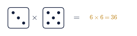
Fig. 390 The multiplication principle. Each of the first die’s \(6\) faces pairs with each of the second die’s \(6\) faces, so the outcomes are not \(6+6\) but \(6\times6=36\) — one for every cell of a \(6\times6\) grid. Independent choices multiply, and this single rule underlies every count in the notebook, including a physical system’s \(g^N\) configurations.#
two dice:           6 × 6     = 36    (enumerated: 36)
three dice:         6 × 6 × 6 = 216   (enumerated: 216)
three-letter words: 26³       = 17576 (enumerated: 17576)
Validation 1#
✓ the multiplication principle's products match brute-force enumeration (36, 216, 17576)
True
Exercise 2 — Permutations versus combinations (worked)#
The first real distinction in counting is whether order matters, and it is worth slowing down on, because it is the source of most counting mistakes. Suppose eight runners finish a race. The number of ways to fill the three podium places — gold, silver, bronze — is a permutation, \(P(8,3)=8\times7\times6=336\), because here the order is the whole point: gold-then-silver is a different outcome from silver-then-gold. But the number of ways to choose a three-person committee from the same eight is a combination, \(C(8,3)=56\), because a committee is just a set — the same three people in any order are the same committee (Fig. 391). The two are related by Eq. 384: a combination is a permutation with the \(k!\) orderings divided back out. Forward-pointer: whether the particles we count are ordered or not is exactly the distinguishable/indistinguishable question we reach in Exercise 9 — the order fork is the classical/quantum fork.
Part a) Compute \(P(8,3)\) with math.perm and \(C(8,3)\) with math.comb.
Part b) Confirm exactly — integer arithmetic, no floating point — that \(C(8,3)=P(8,3)/3!\), the relation Eq. 384 between the two.
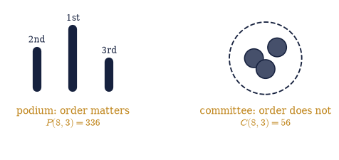
Fig. 391 Order matters, or it does not. Left: filling a podium (gold/silver/bronze) is a permutation — the three places are labelled, so the order of the chosen runners matters, giving \(P(8,3)=336\). Right: choosing a committee is a combination — it is just a set of three, so order is irrelevant and the count drops by the \(3!=6\) orderings to \(C(8,3)=56\). Asking whether order matters is the first and most important fork in all of counting.#
podium finishes (order matters):  P(8,3) = 336
committees (order irrelevant):    C(8,3) = 56
C(8,3) = P(8,3)/3! = 336/6 = 56
Validation 2#
✓ combinations are permutations divided by the k! orderings [got 56 vs expected 56 (rtol=0, atol=1e-09)]
True
Exercise 3 — Socks in a drawer: drawing without replacement (worked)#
Now a count with a probability attached, and our first physical seed. A drawer holds five red and three blue socks, and we pull two out in the dark (Fig. 392). What is the chance both are red? The number of ways to choose any two of the eight socks is \(C(8,2)=28\), and the number of ways to choose two of the five red ones is \(C(5,2)=10\), so the probability is \(10/28\approx0.357\). This is drawing without replacement — the second draw sees a changed drawer — and notice that within a colour the socks are indistinguishable: we count red socks, not which red sock. That is the seed of occupation-number counting, where we ask how many particles occupy a state, not which ones. A matching pair is two red or two blue, so its count is \(C(5,2)+C(3,2)\) — disjoint cases add, where independent choices multiply.
Part a) Compute \(P(\text{two red})=C(5,2)/C(8,2)\) and the probability of a matching pair
with math.comb.
Part b) Verify the two-red probability against a brute-force enumeration of all \(C(8,2)\)
pairs with itertools.combinations: number the socks \(0\)–\(7\) and count the pairs that are
both red.
Part c) Confirm it once more by simulation — draw two socks at random many times with
numpy.random.default_rng (the Setup’s cb.draw_without_replacement) and compare the
observed frequency to the exact count.
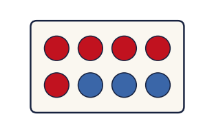
Fig. 392 A drawer of five red and three blue socks. Drawing two in the dark is sampling without replacement: the chance both are red is the number of red pairs over the number of all pairs, \(C(5,2)/C(8,2)=10/28\approx0.357\). Because socks of the same colour are interchangeable, we count how many red, not which red — the seed of occupation-number counting, where a state’s occupancy, not the identity of its occupants, is what matters.#
P(two red)      = C(5,2)/C(8,2) = 10/28 = 0.3571
P(matching pair) = (C(5,2)+C(3,2))/C(8,2) = 0.4643
enumeration over all 28 pairs: P(two red) = 0.3571
Monte Carlo P(two red) over 200,000 draws = 0.3573
Validation 3#
✓  P(two red) from the formula matches the brute-force enumeration of all pairs   [got 0.357143 vs expected 0.357143 (rtol=1e-12, atol=1e-09)]
✓  the Monte Carlo sock-draw frequency matches the exact probability   [got 0.357255 vs expected 0.357143 (rtol=0.03, atol=1e-09)]
True
Exercise 4 — Coins and the binomial coefficient (worked)#
Flip a coin \(n\) times and ask how many of the \(2^n\) possible sequences have exactly \(k\) heads. The answer is the binomial coefficient \(C(n,k)\): choosing which \(k\) of the \(n\) flips are heads is exactly choosing a \(k\)-subset of the \(n\) positions Eq. 384. Stacked up, the counts \(C(n,0),C(n,1),\dots,C(n,n)\) form a row of Pascal’s triangle, and each row sums to \(2^n\) because every sequence has some number of heads (Fig. 393). This is our first two-state system, and it is the combinatorial skeleton of a paramagnet: \(n\) spins each up or down, with \(C(n,k)\) arrangements having \(k\) spins up — the multiplicity we will turn into entropy at §5.4. We work at \(n=6\), whose row is \(1,6,15,20,15,6,1\). Forward-pointer: this two-state count is the paramagnet of §5.4 and the random walk of §5.2.
Part a) Build the Pascal row \(C(n,0),\dots,C(n,n)\) for \(n=6\) with math.comb, and
confirm it sums to \(2^n\) — every sequence has some number of heads.
Part b) Enumerate all \(2^n\) flip sequences explicitly with itertools.product, tally
them by number of heads, and check that the tally reproduces the binomial coefficients.
Pascal row n=6:   [1, 6, 15, 20, 15, 6, 1]
by enumeration:    [1, 6, 15, 20, 15, 6, 1]
row sum = 64 = 2^6 = 64  (every sequence has some k)
Validation 4#
✓ the binomial coefficients count the k-head sequences, and a Pascal row sums to 2^n
True
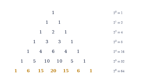
Fig. 393 Pascal’s triangle: row \(n\) holds the binomial coefficients \(C(n,k)\), the number of ways to get exactly \(k\) heads in \(n\) coin flips. Each entry is the sum of the two above it, and each row sums to \(2^n\) (amber, the total number of sequences). Row \(6\) is highlighted — \(1,6,15,20,15,6,1\) — the multiplicities of a six-spin paramagnet, most arrangements clustering near the middle (three up, three down).#
Exercise 5 — Poker hands I: pairs and three of a kind (worked)#
Now the ramp begins, with the structured-counting example everyone has a feel for. A poker hand is five cards from a standard \(52\)-card deck, and the total number of hands is \(C(52,5)=2{,}598{,}960\) — order does not matter, since a hand is a set (Fig. 394). The art is counting hands of a given type by the multiplication principle over independent choices, and we do it slowly here because the method is exactly microstate counting. Take one pair. We choose the rank of the pair (\(13\) ways), choose which two of its four suits appear (\(C(4,2)=6\)), choose three other ranks for the remaining cards (\(C(12,3)=220\)), and choose a suit for each of those three (\(4^3=64\)). Multiplying, \(13\times6\times220\times64=1{,}098{,}240\). Two pair and three of a kind follow the same recipe with the choices regrouped, and the classic values to hit are \(1{,}098{,}240\), \(123{,}552\) and \(54{,}912\). Forward-pointer: “a rarer hand has a smaller count” is the same statement as “a less probable macrostate has fewer microstates” — the heart of §5.4.
Part a) Compute, with math.comb and the choices written out factor by factor, the
counts for one pair, two pair, and three of a kind, and check them against the classic
values.
Part b) Cross-check the one-pair count by dealing hundreds of thousands of random hands
with numpy.random.default_rng (the Setup’s cb.simulate_poker) and comparing the observed
frequency to \(1{,}098{,}240/C(52,5)\).
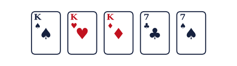
Fig. 394 A five-card poker hand, here a full house (three kings and two sevens). The total number of distinct hands is \(C(52,5)=2{,}598{,}960\), since a hand is an unordered set of five cards. Counting hands of a named type — one pair, a flush — by the multiplication principle over independent choices is precisely the skill of enumerating a physical system’s microstates.#
total hands C(52,5) = 2,598,960
one pair      = 13·C(4,2)·C(12,3)·4³ = 1,098,240
two pair      = C(13,2)·C(4,2)²·11·4 = 123,552
three of a kind = 13·C(4,3)·C(12,2)·4² = 54,912
Monte Carlo P(one pair) = 0.4225 vs exact 0.4226
Validation 5#
✓  the one-pair, two-pair, and three-of-a-kind counts match the classic values   [max|Δ| = 0 (rtol=0, atol=1e-09)]
✓  the Monte Carlo one-pair frequency matches the exact probability   [got 0.422523 vs expected 0.422569 (rtol=0.03, atol=1e-09)]
True
Exercise 6 — Poker hands II: straights and flushes, the subtle ones (worked)#
These are the hands students miscount, so we go carefully. A straight is five cards in consecutive rank. The subtlety is the ace: it plays both high and low, so the runs are \(A2345\), \(23456\), …, up to \(10\,J\,Q\,K\,A\) — ten sequences, not nine (Fig. 395). Each sequence allows any suit for each card, \(4^5=1024\) ways, giving \(10\times1024=10{,}240\). But that total includes the straights that are also all one suit (straight flushes), and a straight flush is a rarer, more special hand we count separately, so we subtract the \(40\) of them: \(10{,}240-40=10{,}200\). A flush is five cards of one suit, \(C(13,5)=1287\) rank-choices per suit times \(4\) suits \(=5148\), again minus the \(40\) straight flushes: \(5{,}108\). The two cautions — the ace wraps, and exclude the overlap — are general microstate-counting discipline.
Part a) Compute the straight-flush count (\(10\) sequences, one suit each) and then the
straight count with math.comb, writing the ace-high-and-low enumeration and the
subtraction of the straight flushes out explicitly. The classic value is \(10{,}200\).
Part b) Compute the flush count the same way — \(C(13,5)\) rank choices per suit, four suits, minus the same \(40\) straight flushes — and confirm the classic \(5{,}108\).
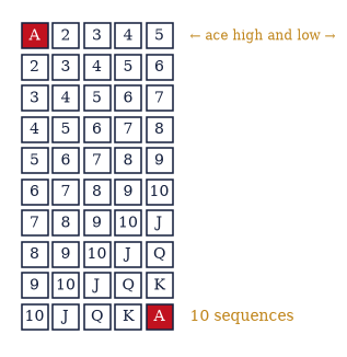
Fig. 395 The ten straights, the subtlety students miss. A straight is five consecutive ranks, and because the ace (A) plays both low (in \(A2345\)) and high (in \(10\,J\,Q\,K\,A\)) there are ten runs, not nine. Each allows \(4^5\) suit choices; subtracting the \(40\) straight flushes (straights that are also one suit, a rarer hand counted separately) gives \(10{,}200\). Excluding overlaps with rarer categories is general microstate-counting discipline.#
straight sequences (ace high AND low): 10
straight = 10·4⁵ − 40 = 10240 − 40 = 10,200
flush    = C(13,5)·4 − 40 = 5148 − 40 = 5,108
Validation 6#
✓ the straight (10 sequences, ace high and low, minus straight flushes) and flush counts are correct [max|Δ| = 0 (rtol=0, atol=1e-09)]
True
Exercise 7 — Poker hands III: the full ranking (worked)#
We finish the ramp by counting the rarest hands and assembling the whole ranking. A full house (three of one rank, two of another) is \(13\times C(4,3)\times12\times C(4,2)=13 \times4\times12\times6=3{,}744\). Four of a kind chooses the rank (\(13\)) and the one outside card (\(48\) remaining), giving \(624\). The straight flush we already have: \(40\). Laid side by side, the counts are the famous ranking of poker hands (Fig. 396), and here is the point worth pausing on: the ranking is by multiplicity. A flush beats a straight, and a flush is rarer than a straight, because there are fewer flushes — \(5{,}108\) against \(10{,}200\). “Rarer” and “stronger” are the same statement, and it is a statement about counts. “High card” is best defined as everything left over, so the completeness check below is a bookkeeping identity rather than an independent test of the eight named counts. Forward-pointer (voice): a system sits in its most probable macrostate for this very reason — that macrostate is the one realised by the most microstates. The ranking of poker hands is a small rehearsal for the second law (§5.3, §5.4).
Part a) Compute the full-house, four-of-a-kind, and straight-flush counts with
math.comb, and check them against \(3{,}744\), \(624\) and \(40\).
Part b) Assemble every category into one census, take high card as the remainder, and confirm that the nine categories sum to \(C(52,5)\).
Part c) Watch the ranking emerge from random dealing: tally tens of thousands of dealt
hands by category (the Setup’s cb.poker_rank) and animate the running frequencies against
the exact probabilities.
full house     = 13·C(4,3)·12·C(4,2) = 3,744
four of a kind = 13·48 = 624
straight flush = 10·4  = 40
high card (the rest)   = 1,302,540
all categories sum to 2,598,960 = C(52,5) = 2,598,960
Validation 7#
✓  the full-house, four-of-a-kind, and straight-flush counts are correct   [max|Δ| = 0 (rtol=0, atol=1e-09)]
✓  every hand is accounted for: the categories sum to C(52,5)
True
We can also watch the counts emerge from random dealing. The animation below deals hands one batch at a time and accumulates the observed frequency of each category, which settles onto the exact probabilities (dark markers) — computation confirming the count (Fig. 396).
Fig. 396 Monte Carlo confirming the counts (animated). Random five-card hands are dealt with numpy.random.default_rng and tallied by category; the bars show the running observed frequency as the number of deals grows, settling onto the exact probabilities computed by hand (dark markers). The rarest hands (left) are so improbable that thousands of deals pass between them — the counting and the simulation agree, as they must.#
Exercise 8 — Stars and bars: indistinguishable objects (worked)#
Here is the hard, beautiful count, and the gateway to quantum statistics. How many ways can \(n\) indistinguishable balls be distributed among \(k\) boxes, with any number allowed per box? The trick is a change of view. Lay the \(n\) balls in a row and insert \(k-1\) bars to divide them into \(k\) groups — the first group goes in box \(1\), the next in box \(2\), and so on (Fig. 397). Every distribution corresponds to exactly one arrangement of stars (balls) and bars, and vice versa, so counting distributions is the same as counting arrangements of \(n+k-1\) symbols of which \(k-1\) are bars:
Because the balls are interchangeable, only how many land in each box matters, not which — precisely the situation for identical bosons among energy states. The three cases below, \((n,k)=(3,2),(5,3),(10,4)\), come out \(4\), \(21\) and \(286\). Forward-pointer: this is the Bose–Einstein count of \(n\) identical particles among \(k\) states (Volume VII).
Part a) Evaluate the stars-and-bars formula \(C(n+k-1,k-1)\) for those three \((n,k)\) with
the Setup’s cb.stars_bars.
Part b) Confirm each value against an explicit enumeration of every distribution, built
with itertools.combinations_with_replacement — a distribution is a multiset of box
labels, which is exactly what that enumerator produces.
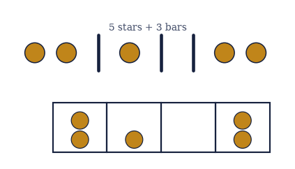
Fig. 397 Stars and bars. To distribute \(n=5\) indistinguishable balls (stars, amber) among \(k=4\) boxes, insert \(k-1=3\) bars (dark) into the row: the balls before the first bar go in box \(1\), the next group in box \(2\), and so on. Every arrangement of \(n+k-1=8\) symbols, \(k-1\) of them bars, is one distribution — so the count is \(C(n+k-1,k-1)=C(8,3)=56\). The bottom row shows the resulting box occupancy. This is the Bose–Einstein count of identical particles among states.#
n= 3 balls, k=2 boxes:  C(4,1) =   4   (enumerated: 4)
n= 5 balls, k=3 boxes:  C(7,2) =  21   (enumerated: 21)
n=10 balls, k=4 boxes:  C(13,3) = 286   (enumerated: 286)
Validation 8#
✓  the stars-and-bars formula matches explicit enumeration of every distribution   [max|Δ| = 0 (rtol=0, atol=1e-09)]
✓  indistinguishable balls in boxes: 4, 21, 286 for (n,k)=(3,2),(5,3),(10,4)   [max|Δ| = 0 (rtol=0, atol=1e-09)]
True
Exercise 9 — The three statistics from one setup (worked)#
This is the centerpiece, and the deepest idea in the notebook. Take one physical question — place \(n\) objects into \(k\) states — and count it three ways, changing nothing but what we assume about the objects Eq. 386. If the objects are distinguishable (each carries an identity, and each independently picks a state), the count is \(k^n\). If they are indistinguishable with any number allowed per state, it is the stars-and-bars \(C(n+k-1,k-1)\). If they are indistinguishable and at most one may occupy a state, it is \(C(k,n)\). For \(n=3\) objects in \(k=5\) states these are \(125\), \(35\), and \(10\) — three different answers to one question (Fig. 398).
These are the three statistics of nature. Distinguishable is Maxwell–Boltzmann (classical particles); indistinguishable-any-number is Bose–Einstein (photons, and any integer-spin particle); indistinguishable-at-most-one is Fermi–Dirac (electrons, and the exclusion principle made into a counting rule). The entire difference between a beam of light and a block of metal is, at this level, a choice of how to count. A reader who has counted poker hands and stars-and-bars can already count quantum states; Volume VII supplies the physics that says which rule applies when. The small case \(n=2\), \(k=3\) is small enough to write out in full, and there the three answers are \(9\), \(6\) and \(3\). Forward-pointer: these three rules are the subject of Volume VII — the photon gas, the electron gas, and Bose–Einstein condensation.
Part a) For \(n=3\), \(k=5\) evaluate all three counts with the Setup’s
cb.count_statistics, and confirm they are \(125\), \(35\), \(10\).
Part b) Enumerate the configurations of the small case \(n=2\), \(k=3\) explicitly — ordered pairs for Maxwell–Boltzmann, multisets for Bose–Einstein, plain subsets for Fermi–Dirac — and check the three lengths, so the reason the counts differ is on the screen rather than in a formula.
n=3 objects, k=5 states — the SAME setup, counted three ways:
  distinguishable (Maxwell–Boltzmann):     kⁿ          = 125
  indistinguishable, any number (Bose–Einstein): C(n+k−1,k−1) = 35
  indistinguishable, ≤1 per state (Fermi–Dirac): C(k,n)      = 10

small case n=2, k=3:  MB=9, BE=6, FD=3
Validation 9#
✓  one setup, three counts: Maxwell–Boltzmann (125), Bose–Einstein (35), Fermi–Dirac (10)   [max|Δ| = 0 (rtol=0, atol=1e-09)]
✓  the small case n=2,k=3 enumerates to MB=9, BE=6, FD=3
True
The enumeration below makes the difference visible. For two objects in three boxes, the distinguishable scheme (left) keeps \(AB\) and \(BA\) as different — nine configurations; the Bose scheme (centre) treats them as the same, collapsing to six; the Fermi scheme (right) additionally forbids two in a box, leaving three (Fig. 398).
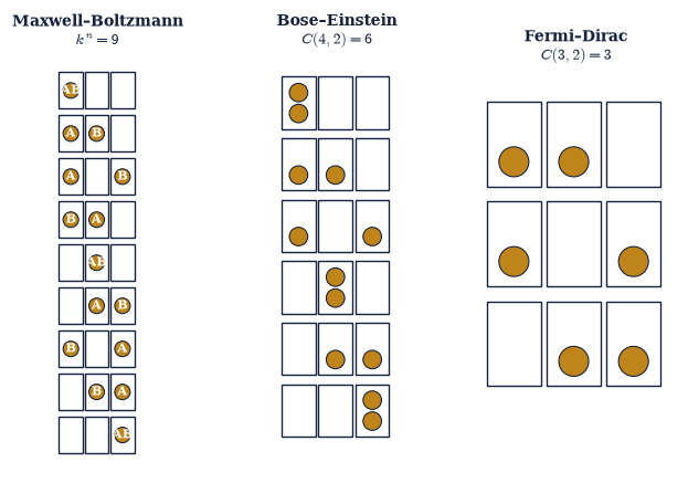
Fig. 398 One setup, three counts (two objects, three boxes). Left, Maxwell–Boltzmann: the objects are distinguishable (\(A\), \(B\)), so \(AB\) and \(BA\) in different boxes are different configurations — \(3^2=9\). Centre, Bose–Einstein: identical objects, any number per box, so order within is meaningless — \(C(4,2)=6\). Right, Fermi–Dirac: identical and at most one per box — \(C(3,2)=3\). Nothing changed but what we assume about the objects, and the count fell from \(9\) to \(6\) to \(3\). At \(n=3,k=5\) the same three rules give \(125\), \(35\), \(10\) — the classical, boson, and fermion counts.#
Exercise 10 — The birthday problem: when counting breaks intuition (student)#
We close with a count whose answer almost everyone gets wrong, as a reminder that careful enumeration beats gut feeling. In a room of \(n\) people, what is the chance that two share a birthday? Intuition says you need many people — there are \(365\) days, after all. But the right count is over pairs, and a room of \(n\) people contains \(C(n,2)\) pairs, which grows fast. It is easier to count the complement: the probability that all birthdays differ is \(\frac{365}{365}\cdot\frac{364}{365}\cdots\frac{365-n+1}{365}\), a multiplication-principle product, and one minus that is the chance of a match. The surprise is that just 23 people already cross \(50\%\) (Fig. 399) — the exact value is \(0.5073\).
Part a) Write birthday_shared(n, days=365), the probability that at least two of \(n\)
people share a birthday. Form the all-distinct product
\(\prod_{i=0}^{n-1}(D-i)/D\) over \(D=\,\)days, which is the multiplication principle applied
to the rooms in which every birthday differs, and return one minus it. Counting the
complement is the whole trick, since the direct count over matching rooms is a nightmare and
this is two lines. Write this one yourself — the implementation is the lesson.
Part b) Evaluate it at \(n=23\) and confirm the probability is just over \(50\%\).
Part c) Cross-check by simulation: generate a hundred thousand random rooms of \(23\)
birthdays with numpy.random.default_rng, count the rooms containing a repeat, and compare
the frequency with Part b).
P(shared birthday, 23 people) = 0.5073 (just over 1/2)
Monte Carlo over 100,000 rooms of 23 = 0.5084
Validation 10#
✓  23 people already give >50% chance of a shared birthday   [got 0.507297 vs expected 0.507 (rtol=0.01, atol=1e-09)]
✓  the Monte Carlo birthday frequency matches the exact probability   [got 0.50844 vs expected 0.507297 (rtol=0.03, atol=1e-09)]
True
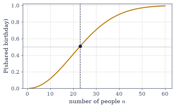
Fig. 399 The birthday problem. The probability that two of \(n\) people share a birthday (amber) climbs far faster than intuition expects, because it counts pairs — of which a room of \(n\) holds \(C(n,2)\). By \(n=23\) (dashed) the chance already exceeds \(50\%\), and by \(n=60\) it is all but certain. Counting the right thing — pairs, not people — is the whole lesson.#
Notebook summary#
Counting is the foundation of statistical mechanics, and this notebook built it from the multiplication principle up to the gateway of quantum statistics.
The multiplication principle Eq. 383: independent choices multiply (\(6\times6=36\)), and a system of \(N\) parts with \(g\) states each has \(g^N\) configurations — microstate counting in embryo.
Permutations and combinations Eq. 384: the order fork, \(P(8,3)=336\) versus \(C(8,3)=56\), with \(C=P/k!\); sampling without replacement (socks, \(C(5,2)/C(8,2)=0.357\)); and the binomial coefficient counting coin sequences (the two-state paramagnet).
Structured counting Eq. 385: the full poker ranking computed exactly and confirmed by Monte Carlo — \(1{,}098{,}240\) pairs down to \(40\) straight flushes — with the ace-high-and-low and exclude-the-overlap subtleties. A rarer hand has a smaller count, the same fact that makes a system sit in its most probable macrostate.
Distinguishability — the tenet Eq. 386: stars-and-bars \(C(n+k-1,k-1)\), and the three statistics from one setup, \(125/35/10\) for \(n=3,k=5\) — Maxwell–Boltzmann, Bose–Einstein, Fermi–Dirac. The classical/quantum distinction is a choice of how to count.
A caution (the birthday problem): \(23\) people already share a birthday with probability \(>1/2\) — count the right thing (pairs), and intuition is no substitute for enumeration.
The same multiplication principle that ranks poker hands enumerates a physical system’s microstates; the distinguishable/indistinguishable fork that separates \(125\) from \(35\) from \(10\) is the very thing that, in Volume VII, separates the photon gas from the electron gas. Counting configurations is the first half of statistical mechanics. The second half is turning those counts into probabilities — which is where §5.2 begins.
Outlook#
Probability (§5.2). From counts to probabilities: distributions, expectation, and variance, in the Born-rule form \(\langle A\rangle\) and the uncertainty \(\Delta A\) that quantum mechanics uses; the binomial, Poisson, and Gaussian distributions.
The large-\(N\) limit (§5.3). Stirling’s approximation, the central limit theorem, and why the most probable configuration overwhelmingly dominates when \(N\sim10^{23}\).
The physics begins (§5.4 onward). Microstate counting becomes entropy \(S=k\ln\Omega\), the Boltzmann distribution, and thermodynamics — emergent, not assumed.
The three statistics in full (Volume VII). The photon (Bose) and electron (Fermi) gases, and Bose–Einstein condensation — the physics behind the three counts established here.
Cross-reference Volume 0 (the computational foundations) and Volume VII (quantum statistics).