


0.1 Floating-Point Arithmetic and Numerical Error#
Notebook overview#
We have spent (probably) years already computing with real numbers: a
mathematically dense continuum, infinitely divisible, and closed under
arithmetic. Yet our computers do not have these mathematical idealisations:
they have instead a finite set of floating-point numbers, a grid with gaps
that thins out as we move away from zero. Every +, -, *, / we have ever
run silently rounded its exact result back onto that grid. Most of the time we
never notice. This notebook is about the times we must.
The material here is not new physics or new mathematics: it is the
computational reality of arithmetic we already trust. We will measure
machine epsilon, the size of the gaps; watch catastrophic cancellation
destroy the quadratic formula and rebuild it; meet the three library
primitives (numpy.expm1, numpy.log1p, scipy.special.logsumexp) that
package that same rewrite and that later volumes treat as compulsory; trace
the U-shaped error
curve of a numerical derivative (one cannot make it arbitrarily accurate by
shrinking the step); tame summation error with compensated addition; and,
finally, explain the number every reader of Volumes I–II has already seen: why
a conserved energy drifts by \(\sim 10^{-11}\) and not by zero. That drift is not
a bug; it is the floor this notebook accounts for.
This is the opening notebook of Volume 0 — Foundations, and it reaches far
forward: the tolerance arguments here are why ecp.validate.close compares
with rtol/atol and never with ==, and the error floor it establishes sits
under every conservation check in the course.
How to read the checks. Each exercise ends with a
validatecall that compares our result to something independent: an exact value, an analytic limit, a known relationship. A ✓ is strong evidence we got it right; a ✗ is not a verdict but a prompt to locate the discrepancy. In a notebook about rounding the point is sharper than usual: the right answer is often “equal to within a tolerance,” never “bit-for-bit equal,” so every check here is itself a small lesson in choosing that tolerance.
Theory in brief#
The IEEE-754 double-precision grid#
A 64-bit double splits its bits into \(1\) sign, \(11\) exponent, and \(52\) mantissa (fraction) bits. A finite (normal) double is
a \(53\)-bit significand (the leading \(1\) is implicit) times a power of two. The representable numbers are therefore not the reals but a finite grid: within each binade \([2^e, 2^{e+1})\) there are exactly \(2^{52}\) equally spaced points, so the absolute spacing doubles every time we cross to the next binade and the grid is far denser near \(0\) than near, say, \(10^8\).
The relative spacing of that grid is the machine epsilon
defined as the gap between \(1\) and the next larger representable double. It is the single most important number in this notebook: it sets the relative resolution of every stored quantity.
The rounding model#
Real arithmetic is not closed on the grid, so every operation rounds its exact result to the nearest representable double. The standard model of this is: for \(\circ \in \{+,-,\times,\div\}\) and the unit roundoff \(u = \varepsilon/2\),
Each individual operation is correctly rounded: accurate to half an ULP (unit in the last place). Trouble comes not from one operation but from how errors propagate and accumulate. The headline consequence: \(0.1\) has no finite binary expansion, so it is stored with a small error, and \(0.1 + 0.2 \ne 0.3\) exactly.
Catastrophic cancellation#
Subtracting two nearly equal numbers is the classic amplifier. If \(a \approx b\) are each accurate to a relative \(\varepsilon\), their stored values carry absolute errors \(\sim \varepsilon|a|\); the difference \(a-b\) is small but inherits those absolute errors, so its relative error blows up by the factor \(|a|/|a-b|\). No leading significant digits survive. The textbook victim is the quadratic formula \(x = (-b \pm \sqrt{b^2-4ac})/2a\) when \(b^2 \gg 4ac\): there \(\sqrt{b^2-4ac} \approx |b|\), and one of the two roots is computed as the difference of two nearly equal numbers.
Truncation versus round-off, and an optimal step#
A numerical derivative trades two errors against each other. The forward difference \(f'(x) \approx \big(f(x+h)-f(x)\big)/h\) has a truncation error \(\sim \tfrac{h}{2}|f''|\) (from the Taylor remainder, shrinking with \(h\)) and a round-off error \(\sim \varepsilon|f|/h\) (the cancellation in the numerator, growing as \(h\) shrinks). Their sum is U-shaped in \(h\) and is minimised at
with a minimum error of order \(\sqrt{\varepsilon}\). (Setting the two error terms equal gives \(h_\star\) in two lines; Press et al., Numerical Recipes, §5.7, carry the analysis out in full.) One cannot make a numerical derivative arbitrarily accurate by taking \(h \to 0\): past \(h_\star\) round-off takes over and the answer gets worse. (A central difference does better: optimum near \(\varepsilon^{1/3}\), error \(\sim \varepsilon^{2/3}\).)
Accumulation and conditioning#
Summing \(N\) terms accumulates rounding: the worst case grows like \(O(N\varepsilon)\), but with errors of random sign the typical growth is a random walk, \(O(\sqrt{N}\,\varepsilon)\). That \(\sqrt{N}\,\varepsilon\) law is the origin of the \(\sim 10^{-11}\) energy drifts we saw in Volumes I–II, now made quantitative. Compensated (Kahan) summation and pairwise summation tame it.
Finally, distinguish a bad algorithm (cancellation: fixable by rewriting) from a badly conditioned problem (intrinsic). The relative condition number \(\kappa\) of evaluating \(f\) at \(x\),
measures how much a relative input perturbation is amplified in the output. (One first-order Taylor expansion of \(f\) delivers both statements; Higham, Accuracy and Stability of Numerical Algorithms, Ch. 1, develops conditioning in full.) Since the input is already stored with a relative error \(\sim\varepsilon\), the best achievable relative accuracy is \(\sim \kappa\varepsilon\): no algorithm can do better. When \(\kappa\) is huge, the problem itself is the limit.
Setup#
Imports and constants only — this notebook’s Setup defines no functions at
all. It holds NumPy and Matplotlib, the decimal module raised to 50 digits
so that later exercises have an independent high-precision yardstick,
scipy.special.logsumexp (one of the three library primitives Exercise 4
measures), and the
two numbers the whole notebook turns on: machine epsilon \(\varepsilon\) and
the unit roundoff \(u = \varepsilon/2\), read from numpy.finfo as reference
values. Everything the notebook is about — measuring \(\varepsilon\) by
experiment, the stable quadratic formula, the error measurements that justify
expm1 and log1p, the difference quotients and their
U-curve, Kahan summation, the round-off random walk, the condition number,
and the fast inverse square root — you build in the exercise where it is
earned.
The Setup below holds this notebook’s data and instruments — nothing you are asked to build. It is collapsed so the building stays yours; expand it whenever you want the details.
machine epsilon  eps = 2.2204460492503131e-16
unit roundoff    u   = 1.1102230246251565e-16
Exercise 1 — The floating-point grid#
The theory says doubles form a finite grid with relative spacing \(\varepsilon\), Eq. 3, that thins out away from zero. This exercise makes all three facts tangible by direct experiment, so that every later “why is this not exactly zero?” has a concrete picture behind it.
Show that \(0.1 + 0.2 \ne 0.3\), and print the exact decimal value stored for \(0.1\) using
decimal.Decimal: the binary expansion of \(0.1\) does not terminate, so it is rounded on input.Find machine epsilon experimentally, as the smallest \(e=2^{-k}\) with \(1+e \ne 1\), and confirm it equals \(\varepsilon\) from Eq. 3 (
numpy.finfo(float).eps).Show the grid spacing scales with magnitude: compare
numpy.nextaftersteps near \(1\) and near \(10^8\).
The schematic in Fig. 5 pictures the non-uniform grid the parts below probe.
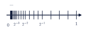
Fig. 5 Schematic of the floating-point grid on \([0,1]\): representable values (ticks) lie \(2^{52}\) to a binade \([2^{e},2^{e+1})\), so the absolute spacing halves at every power of two \(2^{-k}\) (boundaries marked) and the grid bunches toward \(0\). The relative gap is the constant machine epsilon \(\varepsilon\) of Eq. 3; the spacing shown is exaggerated for visibility.#
Solution#
0.1 + 0.2      = 0.30000000000000004
0.3           = 0.29999999999999999
(0.1+0.2)==0.3 ? False
exact stored value of 0.1 = 0.1000000000000000055511151231257827021181583404541015625

experimental eps = 2.2204460492503131e-16
np.finfo eps     = 2.2204460492503131e-16

spacing just above 1     = 2.220e-16
spacing just above 1e8   = 1.490e-08
ratio                    = 6.711e+07  (≈ 1e8)
Validation 1#
✓  experimental machine epsilon matches 2⁻⁵²   [got 2.22045e-16 vs expected 2.22045e-16 (rtol=1e-12, atol=1e-09)]
✓  the grid is coarser near 1e8 than near 1 (spacing scales with magnitude)   [gap(1e8)/gap(1) = 6.711e+07]
True
Exercise 2 — Catastrophic cancellation: the quadratic formula#
This is the centrepiece. The rounding model Eq. 4 guarantees each operation is accurate to half an ULP — yet a sequence of operations can throw away almost every significant digit. The naive quadratic formula \(x = (-b \pm \sqrt{b^2-4ac})/2a\) does exactly this for \(b^2 \gg 4ac\): one root is \((-b + \sqrt{b^2-4ac})/2a\), a subtraction of two nearly equal numbers.
For \(a=1,\ b=10^8,\ c=1\), compute both roots with the textbook formula (
numpy.sqrton the discriminant) and show the small root’s residual \(a x^2 + b x + c\) is far from zero.Write the numerically stable form: compute \(q = -\tfrac12\big(b + \operatorname{sign}(b)\sqrt{b^2-4ac}\big)\) with
numpy.sign, and take \(x_1 = q/a,\ x_2 = c/q\) (Vieta’s \(x_1 x_2 = c/a\) avoids the cancellation). Write this one yourself — the implementation is the lesson.Compare the residuals, and confirm the stable small root matches the analytic small-root limit \(-c/b\). The figure sweeps \(b\) to show the naive relative error climbing while the stable formula stays at the floor.
small root  (naive)  = -100000000   residual = 1.000e+00
small root  (stable) = -1e-08   residual = 1.110e-16
analytic small-root limit -c/b = -1e-08
The figure below sweeps \(b\) over many decades. For each \(b\) we compute the
small root naively and stably, and the relative error against a
50-digit Decimal reference: an independent ground truth.
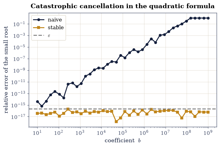
Fig. 6 Relative error of the smaller root of \(x^2 + bx + 1 = 0\) versus the coefficient \(b\), on log–log axes: the naive formula \((-b+\sqrt{b^2-4})/2\) (dark) loses accuracy as \(b\) grows and \(b^2 \gg 4\) drives catastrophic cancellation, while the algebraically stable form \(x_2 = c/q\) (amber) holds at the machine-epsilon floor \(\varepsilon\) (dashed). Error is measured against a 50-digit reference.#
Validation 2#
✓  the stable formula recovers the small root (≈ -c/b)   [got -1e-08 vs expected -1e-08 (rtol=1e-09, atol=1e-09)]
✓  the naive small root has a large residual; the stable one does not   [|res_naive| = 1.000e+00,  |res_stable| = 1.110e-16]
True
Exercise 3 — Loss of significance in a familiar identity#
A “new look” at something we have differentiated a hundred times. The function \(g(x) = \dfrac{1 - \cos x}{x^2}\) tends to \(\tfrac12\) as \(x\to0\) — but evaluated naively near \(0\) it is noise, because \(1-\cos x\) is a subtraction of two numbers both \(\approx 1\) (cancellation again, per Eq. 4). The cure is algebra, not a smaller step: using \(1-\cos x = 2\sin^2(x/2)\),
which has no cancellation.
Implement both forms.
On a log-spaced \(x\) (
numpy.logspace), show the naive form disintegrates into hash as \(x\to0\) while the stable form rides smoothly to \(\tfrac12\).Confirm the stable form equals \(\tfrac12\) to a tight tolerance at very small \(x\), where the naive form cannot.
at x = 1.0e-12: stable = 0.5, naive = 0
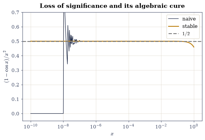
Fig. 7 The function \(g(x)=(1-\cos x)/x^2\) near the origin, evaluated two ways on a logarithmic \(x\)-axis: the naive form (dark) collapses into round-off hash for \(x \lesssim 10^{-3}\) as \(1-\cos x\) cancels, then drops to \(0\) once \(\cos x\) rounds to \(1\); the algebraically equivalent form \(\tfrac12(\sin(x/2)/(x/2))^2\) (amber) rides smoothly to its limit \(\tfrac12\) (dashed).#
Validation 3#
✓  the stable form → 1/2 as x→0   [max|Δ| = 4.17444e-14 (rtol=1e-06, atol=1e-10)]
✓  the naive form fails to reach 1/2 at tiny x (it is dominated by round-off)   [naive(x=1e-12) = 0]
True
Exercise 4 — The library already did the algebra: expm1, log1p, logsumexp#
Exercises 2 and 3 cured cancellation by hand, with a substitution borrowed from Vieta and a half-angle identity. That works, and it scales exactly as far as our patience does. A handful of cancellations recur so relentlessly that the rewrite ships with the library instead, and this course leans on three of them hard enough that they are worth measuring once, here, while the disease is fresh.
The first is \(e^x - 1\) at small \(x\). Since \(e^x = 1 + x + O(x^2)\), the stored value of \(e^x\) is \(1\) plus a few low-order bits, so subtracting \(1\) is precisely the amplifier of Eq. 4: the absolute error of \(\mathrm{fl}(e^x)\) is \(\sim u\) however small \(x\) becomes, the difference inherits that absolute error intact, and the relative error is therefore
which reaches \(100\%\) once \(x\) falls to \(\sim\varepsilon\). numpy.expm1
evaluates \(e^x-1\) as a single correctly rounded operation, from a series whose
leading term is \(x\), so nothing ever cancels. Its twin numpy.log1p does the
same for \(\ln(1+x)\), where the damage is done one step earlier still:
\(\mathrm{fl}(1+x)\) discards the low bits of \(x\) before the logarithm is
called, the same input rounding Exercise 1 exhibited for \(0.1\).
The third is a cousin rather than a twin. Statistical mechanics needs
\(\ln\sum_i e^{a_i}\) constantly, and written that way it overflows to inf the
moment any \(a_i\) passes \(\approx 709\), even when the answer is an unremarkable
number. scipy.special.logsumexp factors the largest exponent out first,
\(\ln\sum_i e^{a_i} = a_{\max} + \ln\sum_i e^{a_i - a_{\max}}\), so no exponential
it evaluates ever exceeds \(1\). The failure mode is overflow rather than
cancellation, but the moral is the one this notebook keeps making: the formula
that is correct in \(\mathbb{R}\) and the formula one hands to a machine are
different formulas.
None of this is decoration. Every Planck and Bose denominator in Volume VII
goes through numpy.expm1 as a standing rule
(§7.5,
§7.14), and the
partition-function recursions of
§5.8 and
§7.17
run entirely in logarithms through logsumexp. This exercise is where those
rules are earned rather than announced.
Sweep \(x = 10^{-1}, 10^{-2}, \dots, 10^{-16}\) (
numpy.logspace) and evaluate \(e^x-1\) both ways, naively asnumpy.exp(x) - 1.0and asnumpy.expm1(x). Form each one’s relative error against a 50-digit reference,Decimal(x).exp() - 1, and confirm the naive error tracks the envelope \(\varepsilon/|x|\) of Eq. 7 whileexpm1holds the floor.Repeat for \(\ln(1+x)\):
numpy.log(1.0 + x)againstnumpy.log1p(x), referenced to(Decimal(1) + Decimal(x)).ln().Exhibit the overflow. For \(a = (1000, 1001, 1002)\) evaluate
numpy.log(numpy.sum(numpy.exp(a)))insidenumpy.errstate(over="ignore")(the overflow is the demonstration, not an accident) and compare withscipy.special.logsumexp(a), checked against the hand-shifted value \(1002 + \operatorname{log1p}(e^{-1} + e^{-2})\) — which is Part 2’s primitive doing the last step safely.
Fig. 8 puts both error sweeps side by side.
at x = 1e-16:
  e^x−1   naive rel. err 1.000e+00,  expm1 5.000e-17
  ln(1+x) naive rel. err 1.000e+00,  log1p 5.000e-17
worst library error over the whole sweep: 1.051e-16  (u = 1.110e-16)

naive log(sum(exp(a))) = inf
scipy logsumexp(a)     = 1002.4076059644444
hand-shifted reference = 1002.4076059644444
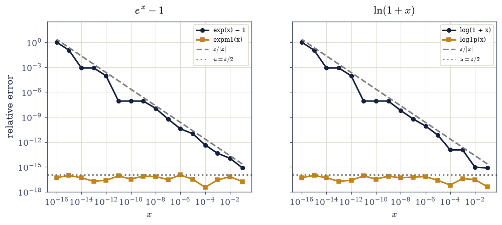
Fig. 8 Relative error of \(e^x-1\) (left) and \(\ln(1+x)\) (right) versus \(x\) on log–log axes, measured against a 50-digit reference. Evaluated naively as \(\exp(x)-1\) and \(\log(1+x)\) (dark) the error climbs along the envelope \(\varepsilon/|x|\) (dashed) of Eq. 7 until every significant digit is gone at \(x\sim10^{-16}\); numpy.expm1 and numpy.log1p (amber) hold the unit-roundoff floor \(u=\varepsilon/2\) (dotted) across all sixteen decades.#
Validation 4#
✓  expm1 and log1p keep full relative accuracy across all sixteen decades   [max|Δ| = 1.05053e-16 (rtol=1e-06, atol=8.88178e-16)]
✓  the naive forms lose every significant digit at x = 1e-16 (relative error ~1)   [exp(x)−1: 1,  log(1+x): 1]
✓  logsumexp returns the exact shifted value where the naive log-sum-exp overflows to inf   [naive = inf, logsumexp = 1002.4076059644, reference = 1002.4076059644]
True
Exercise 5 — Numerical differentiation and the error U-curve#
Recall the trade-off behind Eq. 5: the forward-difference derivative carries a truncation error \(\sim \tfrac{h}{2}|f''|\) that shrinks with \(h\) and a round-off error \(\sim \varepsilon|f|/h\) that grows as \(h\to0\). Their sum is U-shaped, minimised at \(h_\star \sim \sqrt{\varepsilon}\). This is the canonical demonstration that smaller is not always better.
For \(f=\sin\) at \(x=1\) (so \(f'=\cos 1\) is the exact target), sweep \(h\) over many decades (
numpy.logspace) and plot the forward-difference error: the signature U.Confirm the empirical optimum \(h_\star\) (
numpy.argminof the error) matches \(\sqrt{\varepsilon}\) from Eq. 5.Add the central difference and show its optimum sits near \(\varepsilon^{1/3}\) with a markedly lower minimum error.
This points forward: it is why the integrators in §1.6 (and every ODE solve in the course) have a sweet-spot step rather than an arbitrarily small one.
forward-difference optimum h* = 3.969e-09   (√ε = 1.490e-08)
central-difference optimum h* = 5.039e-06   (ε^(1/3) = 6.055e-06)
min error: forward = 4.775e-10,  central = 9.612e-13
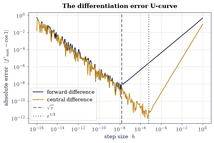
Fig. 9 Absolute error of numerical derivatives of \(f=\sin\) at \(x=1\) versus step size \(h\), on log–log axes — the signature error U. The forward difference (dark) falls with truncation slope \(\sim h\) until round-off \(\sim\varepsilon/h\) takes over near \(h_\star\sim\sqrt{\varepsilon}\) (dashed vertical); shrinking \(h\) further makes the answer worse. The central difference (amber) bottoms out lower, near \(\varepsilon^{1/3}\) (dotted vertical).#
Validation 5#
✓  the forward-difference optimum is h* ~ √ε (within a decade)   [h* = 3.97e-09,  √ε = 1.49e-08  (0.57 decades off)]
✓  the central difference reaches a lower minimum error than the forward difference   [min central 9.61e-13 < min forward 4.77e-10]
True
Exercise 6 — Summation error and compensated summation#
Adding many numbers accumulates the per-operation rounding of Eq. 4. Summing \(N\) copies of \(0.1\) should give \(0.1N\); naively it does not, and the error grows with \(N\).
Sum \(10^6\) copies of \(0.1\) sequentially (a plain Python loop) and measure the error against the exact value \(10^5\).
Write Kahan (compensated) summation, which carries a running correction for the lost low-order bits, and show it is accurate to the floor. Write this one yourself — the implementation is the lesson.
Compare against
numpy.sum, which already uses pairwise summation (it splits the array and recurses), so its error grows like \(O(\log N)\) rather than \(O(N)\). The figure sweeps \(N\) to show the three growth laws.
naive sequential  error = 1.333e-06
Kahan compensated error = 0.000e+00
NumPy pairwise    error = 2.910e-11
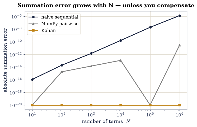
Fig. 10 Absolute error of summing \(N\) copies of \(0.1\) against the exact value \(0.1N\), versus \(N\) on log–log axes: naive sequential addition (dark) accumulates error that climbs roughly \(\propto N\), NumPy’s pairwise np.sum (grey) grows only \(\sim\log N\), and Kahan compensated summation (amber) stays at the floor where the only residue is the input rounding of \(0.1\) itself.#
Validation 6#
✓ Kahan summation eliminates the naive accumulation error [naive 1.33e-06 vs Kahan 0.00e+00]
True
Exercise 7 — Why physics energy drifts are ~1e-11, not 0#
Here is the payoff that ties this notebook to all of mechanics. Throughout Volumes I–II we validated integrators by watching a conserved energy stay flat. It never stayed exactly flat, though; it drifted at the \(10^{-11}\) level. That floor is the \(\sqrt{N}\,\varepsilon\) accumulation of the rounding model, and we can isolate it cleanly. Our bare-rotation demo does far less arithmetic per step than a real adaptive solver, so its floor lands about two orders below the \(10^{-11}\) of Volumes I–II — yet it follows the identical \(\sqrt{N}\,\varepsilon\) law, which is the point.
Take the simple harmonic oscillator \(\ddot x = -\omega^2 x\). Its exact time-\(\Delta t_n\) propagator is a rotation in the \((x,\,v/\omega)\) plane,
which conserves \(E = \tfrac12(v^2 + \omega^2 x^2)\) exactly in real
arithmetic, for any steps \(\Delta t_n\): there is zero truncation error.
So when we iterate it in floating point, any drift in \(E\) is pure
round-off. We use irregular steps \(\Delta t_n\) (exactly what an adaptive
solver like the DOP853 of Volumes I–II does), which makes the per-step
rounding error random in sign; over \(N\) steps it random-walks to
\(\sim\sqrt{N}\,\varepsilon\) rather than cancelling or growing linearly. (With a
single fixed step the rounding bias is systematic and the drift instead grows
\(\propto N\); irregular steps are the realistic case.)
Iterate the exact rotation propagator for \(2\times10^5\) irregular steps (step sizes drawn with
numpy.random.default_rng), recording the relative energy error \(|E_N - E_0|/E_0\) every thousand steps.Plot the accumulated error against \(N\) on log–log axes — the right view for a power law, where the walk and its \(\sqrt{N}\,\varepsilon\) envelope read as parallel lines.
Confirm the error stays at the floating-point floor and grows far slower than the worst-case \(N\varepsilon\).
after N = 200,000 steps:  relative energy error = 3.442e-14
√N·ε round-off floor          = 9.930e-14   (worst case N·ε = 4.441e-11)
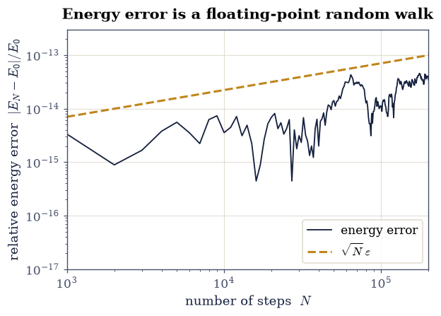
Fig. 11 Relative energy error \(|E_n-E_0|/E_0\) of an exact rotation propagator for the harmonic oscillator taking irregular time steps (zero truncation error), accumulating over \(N\) steps on log–log axes: the trace (dark) random-walks upward parallel to the \(\sqrt{N}\,\varepsilon\) envelope (dashed), demonstrating that the residual is pure floating-point round-off — the same floor under every energy-conservation check in Volumes I–II.#
Validation 7#
✓  energy error stays at the floating-point accumulation floor (~√N·ε)   [error 3.44e-14  at the √N·ε floor 9.93e-14  (checked with ×100 head-room)]
✓  the error grows far slower than the worst-case linear N·ε (it is a random walk)   [error 3.44e-14  vs  N·ε = 4.44e-11]
True
Exercise 8 — Conditioning: when the problem, not the algorithm, limits us (student animation)#
Cancellation in Exercises 2–3 was a fixable defect of the algorithm: rewrite the formula and the error vanishes. Some problems are not so kind: a badly conditioned problem amplifies error no matter how cleverly one computes it, because the input is already stored with a relative error \(\sim\varepsilon\) and Eq. 6 multiplies it by \(\kappa\). The achievable accuracy is \(\sim\kappa\varepsilon\), full stop.
Take \(f(x)=\tan x\) near \(x=\pi/2\), where \(\kappa(x) = |x f'/f| = |2x/\sin 2x|\) diverges.
Compute \(\kappa(x)\) analytically, and measure the amplification by perturbing the input by a small relative \(\delta\) and forming \((\,|\tan(x(1+\delta))-\tan x|/|\tan x|\,)/\delta\) with
numpy.tan.You build the animation: as \(x \to \pi/2\), animate the measured amplification climbing along the analytic \(\kappa(x)\) curve (and the achievable-accuracy floor \(\kappa\varepsilon\) rising with it). Use
FuncAnimation,plt.close(fig), thenecp.animate.show.Confirm the measured amplification tracks \(\kappa\), so the relative error indeed tracks \(\kappa\varepsilon\).
Because the check tests the data (amplification vs. \(\kappa\)), a ✗ means “re-examine the condition-number formula or the perturbation measurement,” never “the animation is wrong.”
κ ranges from 14.8 to 4.97e+04
max |amp/κ - 1| = 4.977e-05
Now build the animation (Part b). The data are ready: xs, kappa,
amp_measured, and the floor. Sweep a marker along the curve as \(x\to\pi/2\).
Fig. 12 Animation of the conditioning of \(f(x)=\tan x\) as \(x\to\pi/2\): the analytic relative condition number \(\kappa(x)=|2x/\sin 2x|\) (dark) and the measured amplification of a small relative input perturbation (amber markers) both diverge and coincide, while the achievable-accuracy floor \(\kappa\varepsilon\) (dashed) rises in step — past a point the problem itself, not the algorithm, sets the error.#
Validation 8#
✓ the measured relative-error amplification equals the condition number κ [max|Δ| = 2.47209 (rtol=0.01, atol=1e-09)]
True
Exercise 9 — Practical hygiene (synthesis)#
A short, rigorous wrap-up of the rules every later notebook leans on.
Never test floats with
==. \(0.1+0.2 \ne 0.3\), yet they agree to within a few \(\varepsilon\). Compare with a tolerance: exactly whatecp.validate.close(got, expected, rtol=…, atol=…)does, and why it exists.rtolvsatol. A check passes when \(|{\rm got}-{\rm expected}| \le {\tt atol} + {\tt rtol}\,|{\rm expected}|\). Usertolfor quantities with a natural scale (energies, frequencies) andatolfor quantities that should be near zero (a residual, a drift), where a relative test is meaningless.Reach for more precision only when one must, and know its cost.
math.fsumsums exactly (at \(O(N)\) bookkeeping);decimalandmpmathgive arbitrary precision but run orders of magnitude slower: fine for a reference value (as in Exercise 2), not for an inner loop.
The check below states rule 1 as code: the two numbers are not equal, yet they are equal to within a tolerance.
✓ float equality needs tolerances, not == (0.1+0.2 ≠ 0.3, but within a few ε) [|0.1+0.2-0.3| = 5.551e-17]
True
Exercise 10 — Showpiece: the fast inverse square root#
One last flourish, because it is the most beautiful thing floating-point bit layout has ever bought. Three-dimensional graphics normalise vectors without pause: every lighting and reflection calculation needs \(\hat{\mathbf v} = \mathbf v / \lVert\mathbf v\rVert\), which is \(1/\sqrt{x}\) with \(x = v_x^2 + v_y^2 + v_z^2\), evaluated millions of times per frame. In the 1990s, before CPUs carried a fast hardware square root, the Quake III Arena source did it with a fragment that became legendary the instant people read it:
i  = 0x5f3759df - ( i >> 1 );               // what the f***?
y  = y * ( 1.5f - ( 0.5f * x * y * y ) );   // 1st iteration
(the bewildered comment is in the original). It returns \(1/\sqrt{x}\) to a fraction of a percent using no division and no square root, only an integer subtraction, a bit shift, and one multiply-heavy polish step. The entire trick is the floating-point representation that this whole notebook has been about.
Why it works (the conceptual centre). Recall the IEEE-754 layout from the
start of this notebook: a float stores a sign, an exponent, and a mantissa, and
for \(x = 2^e(1+m)\) the integer read straight off those same bits is, up to
scaling, an affine function of \(\log_2 x\). At an exact power of two the
relationship is not approximate but exact: reading the float32 bits of
\(x = 2^e\) as an integer \(I\) gives \(I/2^{23} - 127 = e = \log_2 x\) on the nose,
because the mantissa field is zero and only the exponent contributes. Part b)
checks this. Since the bits essentially are \(\log_2 x\), halving and negating
them computes \(-\tfrac12\log_2 x = \log_2\!\big(x^{-1/2}\big)\), which is the bit
pattern of \(1/\sqrt{x}\). The magic constant 0x5f3759df is the additive
correction that best re-centres the affine approximation across the mantissa and
restores the exponent bias.
The polish. The bit hack alone is good to about \(3.4\%\). One step of Newton’s method applied to \(f(y) = 1/y^2 - x\) (whose positive root is \(1/\sqrt{x}\)) gives the update \(y \leftarrow y\,(1.5 - 0.5\,x\,y^2)\) and drops the error to the famous \(\sim0.17\%\); a second step reaches \(\sim10^{-6}\). This is a first sighting of Newton’s method, the subject of §0.2, its quadratic convergence already doing real work.
Write it on
float32, using.view(np.int32)and.view(np.float32)for the bit reinterpretation, with the magic constant stated explicitly. Write this one yourself — the implementation is the lesson.Verify the bits-are-\(\log_2\) identity exactly at \(x = 1,2,4,8,16\): the heart of the matter.
Measure the maximum relative error with the magic step only, with one Newton step, and with two, across a range of \(x\) (Fig. 13).
fast_inv_sqrt(2) = 0.706930 (exact 1/√2 = 0.707107)
Part b) the centre of the whole trick: at exact powers of two the integer read off the bits equals \(\log_2 x\) with no error, so the bit pattern carries the logarithm the algorithm exploits.
   x     bits/2²³ − 127     log₂(x)
    1        0.000000          0.0
    2        1.000000          1.0
    4        2.000000          2.0
    8        3.000000          3.0
   16        4.000000          4.0
Part c) sweep \(x\) and measure the relative error against the exact float64
value, with zero, one, and two Newton steps.
max relative error  magic only = 3.4373%
max relative error  +1 Newton  = 0.1752%
max relative error  +2 Newton  = 4.66e-06
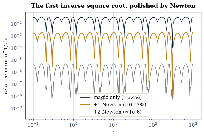
Fig. 13 Relative error of the fast inverse square root for \(1/\sqrt{x}\) versus \(x\), on log–log axes: the bit-hack initial guess alone (dark) stays under \(\approx3.4\%\) across every octave, one Newton step (amber) drops it to the famous \(\approx0.17\%\), and a second step (grey) reaches \(\sim10^{-6}\), near the float32 floor. The error pattern repeats each octave because the underlying approximation is periodic in \(\log_2 x\).#
The lesson behind the spectacle: a representation trick, exploited honestly, had enormous practical impact. Normalising vectors for lighting and reflection is so ubiquitous in real-time graphics that shaving the cost of \(1/\sqrt{x}\) helped make games like Quake III run at all on 1990s hardware. The bits of a float are not an opaque encoding; they are, quite literally, almost a logarithm.
Validation 10#
✓  the integer bit value equals log₂(x) exactly at powers of two (why the trick works)   [max|Δ| = 0 (rtol=1e-06, atol=1e-06)]
✓  one Newton step brings the fast inverse sqrt to ~0.17% error   [got 0.00175198 vs expected 0.00175 (rtol=1e-06, atol=0.0005)]
True
Notebook summary#
The floating-point grid and machine epsilon (\(\approx2.2\times10^{-16}\) for float64); catastrophic cancellation in the naive quadratic formula and loss of significance, and their stable rewrites.
The same rewrites packaged as library primitives: naive \(e^x-1\) and \(\ln(1+x)\) lose every digit by \(x\sim10^{-16}\), tracking \(\varepsilon/|x|\), while
numpy.expm1andnumpy.log1phold a relative error below \(u=\varepsilon/2\) across sixteen decades, andscipy.special.logsumexpreturns \(1002.4076059644\) where \(\ln\sum e^{a_i}\) overflows toinf— the reason Volumes V and VII make all three compulsory.The numerical-differentiation error U-curve (truncation versus round-off, optimal step \(h\sim\sqrt\epsilon\)); compensated (Kahan) summation; why physics energy drifts sit near \(10^{-11}\), not zero; conditioning; and the fast inverse square root as a showpiece.
Outlook#
The rest of IEEE-754: subnormals (gradual underflow), \(\pm\infty\), signed zero, and
NaN: including whyNaN != NaNis by design (it makes “is this a number?” testable asx != x).Interval arithmetic, which carries rigorous error bars through a whole computation instead of a single rounded value.
float32vsfloat64: the speed/memory/accuracy trade behind GPU physics and machine learning, where halving precision doubles throughput.Symbolic computation (SymPy) as the escape hatch from rounding entirely: exact at the cost of speed. We will use it to derive equations of motion in §2.1 rather than to evaluate them.