


1.8 The Solar System: N-Body Gravitation and the Long Game#
Notebook overview#
§1.4 solved the two-body problem and closed it with a theorem: bound orbits are ellipses, fixed in space, forever. The real solar system violates that theorem everywhere, gently: every planet pulls on every other, ellipses precess, and the question of whether the whole arrangement is stable resisted the greatest analysts of three centuries before becoming, in the 1980s, a question for computers [Las89]. This notebook builds the full N-body problem: all eight planets and the Sun, one force law, no approximations beyond the discretization of time.
Two threads from earlier notebooks come due. First, the integrator lesson of §1.6: over a thousand years the difference between a symplectic method and a “better” adaptive one is not accuracy but character, bounded energy wobble versus secular drift, and we measure both. Second, the Mercury thread: §2.4 explains why a perturbed orbit precesses and Volume IV’s capstone computes relativity’s famous 43 arcseconds per century; here we compute the much larger Newtonian share, the ~530 arcseconds per century that Mercury’s perihelion drifts because Venus, Jupiter, and the rest exist, and assemble the historical ledger those numbers settle. The craft on display is measurement discipline: our integrator precesses orbits numerically, so we measure that bias on a problem whose answer is exactly known (the two-body system: zero) and subtract it. The standard reference for everything deeper is Murray & Dermott [MD99].
A note on reading the checks in this notebook: a validation compares a result to an expected physical fact. A ✗ does not by itself mean the answer is wrong; it means the output did not match what the check expected, which may be a genuine error, a different-but-valid convention, or too tight a tolerance. Treat a ✗ as a prompt to locate the discrepancy. Passing is strong evidence, not proof.
Theory in brief#
The N-body problem. Bodies \(i = 0, \dots, N-1\) with masses \(m_i\) at positions \(\mathbf r_i\) obey
pairwise inverse-square attraction and nothing else. Total energy, momentum, and angular momentum are conserved exactly; almost nothing else is. For \(N \ge 3\) there is no general closed-form solution, which is why this notebook exists.
Astronomical units. Measuring length in AU, time in years, and mass in solar masses makes the numbers tame and fixes \(G\): for a test mass on a circular orbit of radius \(1\) AU and period \(1\) yr, Kepler’s third law \(T^2 = 4\pi^2 a^3 / G M_\odot\) forces
Building orbits from elements. An orbit of semi-major axis \(a\) and eccentricity \(e\) has perihelion distance \(r_p = a(1 - e)\), and the vis-viva equation \(v^2 = G(M + m)(2/r - 1/a)\) gives the perihelion speed
perpendicular to the radius. Launching each planet at its perihelion with Eq. 131 builds a model solar system, coplanar, with each planet’s real \((a, e)\) but arbitrary perihelion directions: the right masses, sizes, and shapes, without pretending to be an ephemeris. For the secular (orbit-averaged) questions this notebook asks, that is the physics that matters.
Symplectic integration and the long game. §1.6 showed velocity Verlet’s energy error oscillating while Euler’s grew; the deep reason is that Verlet is symplectic (it exactly conserves a slightly-wrong Hamiltonian, so the energy of the true one can only wobble). Adaptive Runge–Kutta is more accurate per step and not symplectic: its small per-step energy errors accumulate with one sign, a secular drift that no tolerance setting removes, only postpones. For a thousand-year integration the distinction is the whole game.
Precession and the LRL vector. For pure \(1/r\) attraction the Laplace–Runge–Lenz vector of §1.4,
(per unit mass, heliocentric) is a constant pointing at perihelion, so its angle is a precession meter: any secular rotation of \(\mathbf A\) measures departure from closed ellipses, whether caused by other planets (real) or by the integrator (artifact). The perturbing planets drive Mercury’s perihelion forward at a rate classical secular theory puts near \(532''\)/century (Venus \(\approx 278\), Jupiter \(\approx 154\), Earth \(\approx 90\), the rest small); general relativity adds \(43''\) (§4.8); together they close the observed budget that once had astronomers hunting for the phantom planet Vulcan.
Setup#
Masses (in \(M_\odot\)), semi-major axes (AU), and eccentricities for the
eight planets are the standard fact-sheet values. Everything integrates in
the barycentric frame (total momentum removed); heliocentric quantities are
differences from the Sun’s state. This notebook’s own machinery is not
here: you write the N-body force law nbody_accel in Exercise 1 and the
system launcher build_system in Exercise 2. What Setup holds besides the
data is instruments — the velocity Verlet driver of
§1.6 and the LRL angle meter of
§1.4, both built from scratch there and restated
here, plus an energy diagnostic and a unit conversion. No randomness
appears anywhere in this notebook.
The Setup below holds this notebook’s data and instruments — nothing you are asked to build. It is collapsed so the building stays yours; expand it whenever you want the details.
Exercise 1 — One force law, written and certified#
Everything downstream rests on the force law, so the notebook’s first build is its most consequential — and the certification that follows it spends two answers known in advance. The unit system Eq. 130 fixes \(G = 4\pi^2 = 39.4784\ldots\) exactly by construction, so a test mass on a one-AU circular orbit must feel exactly that acceleration, directed at the Sun; and §1.4’s closed-orbit theorem says that orbit returns to where it started after exactly one period, which in these units is one year. Machinery is only worth trusting with nine bodies once it has reproduced answers that were already known.
Part a) Write nbody_accel(m, r), returning all \(N\) accelerations of
Eq. 129 at once: build the \((n, n, 2)\) array of separations
\(\mathbf r_j - \mathbf r_i\), the \((n, n)\) inverse-cube distances with the
diagonal zeroed (a body does not pull on itself), and contract against
the masses — \(O(N^2)\) pairwise gravity with no Python loop over pairs.
Write this one yourself — the implementation is the lesson.
Part b) Verify the unit system: confirm that a test mass
(\(m = 10^{-12}\,M_\odot\)) on the circular orbit \(r = (1, 0)\) AU,
\(v = (0, 2\pi)\) AU/yr around a solar mass at the origin feels acceleration
of magnitude exactly \(G\) from nbody_accel (rtol=1e-12), pointing in
\(-\hat{\mathbf x}\).
Part c) Integrate that two-body system for one year with the Setup’s
verlet_orbits — which now drives the nbody_accel you just wrote — at
\(\Delta t = 10^{-4}\) yr and verify the test mass returns to its starting
point to within \(|\Delta \mathbf r| < 10^{-5}\) AU: the definition of the
year, recovered by the machinery that will now be pointed at the real
system.
G = 4π² : 39.478418; |a| on the unit circle: 39.478418
orbit closure: 8.27e-07 AU after one year
✓ on the unit circular orbit the acceleration magnitude is exactly G = 4π², the unit system's defining identity [got 39.4784 vs expected 39.4784 (rtol=1e-12, atol=1e-09)]
✓ and it points at the Sun: pure −x̂ at (1, 0) [a = (-39.4784, 0.0e+00)]
✓ the circular orbit closes after exactly one year: the year, recovered [|Δr| = 8.27e-07 AU]
True
Exercise 2 — Nine bodies, five years#
Now the whole system — which first has to exist.
Part a) Write build_system(names=None): assemble the Sun and the
selected planets (default: all eight), launching each planet at its
perihelion distance \(a(1-e)\) with the vis-viva speed Eq. 131
perpendicular to the radius (Fig. 105 shows the
construction for one orbit). Spread the perihelion directions by the
golden angle \(\pi(3-\sqrt{5})\) so no artificial alignment biases the
perturbations, and shift the whole system to the barycentric frame
(total momentum and centre of mass removed), so the Sun wobbles as it
truly does. Return (m, r, v) with index \(0\) the Sun.
Part b) Certify the launcher through the conservation laws, on a
two-planet system it assembles (Sun, Earth, Jupiter;
\(\Delta t = 5 \times 10^{-4}\) yr, \(20\) yr): total energy from
total_energy conserved to \(|\Delta E/E| < 10^{-8}\), total momentum
\(\sum m\mathbf v\) zero to \(10^{-12}\) (it started zero and Verlet’s
pairwise forces cannot create any), and total angular momentum
\(\sum m (x v_y - y v_x)\) conserved to relative \(10^{-10}\).
Part c) Integrate the full nine-body system with verlet_orbits for
\(5\) yr at \(\Delta t = 10^{-4}\) yr (sampling every 100 steps) and verify
total energy is
conserved to \(|\Delta E/E| < 10^{-8}\) and the barycentre stays put
(\(|\sum m \mathbf r|/M_{\rm tot} < 10^{-10}\) AU): with every planet
pulling on every other, the conservation laws are the only guarantee not
negotiated away.
Part d) Plot the orbits (inner system and full system panels), and animate the inner four planets with fading trails: five years is four Mercury years plus a bit, and genuine motion is exactly what a still cannot show. The animation’s physics is validated through Part c)’s conserved quantities, which are computed from the same trajectory the player draws.
|ΔE/E| max : 6.05e-09
|P| final : 2.61e-17
|ΔL/L| max : 3.99e-14
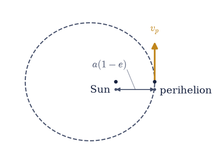
Fig. 105 The perihelion-launch construction of the model solar system, for one orbit: the planet starts at perihelion distance \(a(1-e)\) from the Sun (ink dot at the focus) with the vis-viva speed \(v_p=\sqrt{G(M_\odot+m)(1+e)/(a(1-e))}\) directed perpendicular to the radius (amber arrow), which reproduces exactly the ellipse of semi-major axis \(a\) and eccentricity \(e\) (dashed).#
|ΔE/E| over 5 yr : 3.80e-09
barycentre drift : 1.90e-16 AU
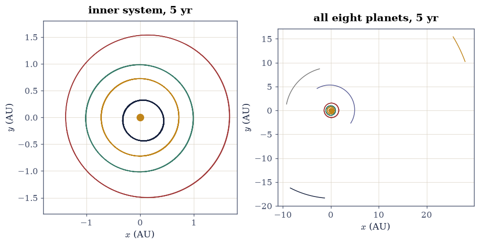
Fig. 106 Five years of the nine-body model solar system, integrated with velocity Verlet at \(\Delta t=10^{-4}\) yr, in the barycentric frame. Left: the inner system (Mercury through Mars), each planet completing between five and one-third orbits; right: the full system, where the giant planets have barely moved and the inner orbits blur into their tracks. The Sun’s barycentric wobble is real but invisible at this scale.#
Fig. 107 Animation of the inner solar system’s five integrated years: Mercury, Venus, Earth, and Mars (amber to ink) orbit the barycentric Sun with month-long fading trails. Mercury laps the field while Mars completes under three orbits; the frame is the barycentre, so the Sun itself wobbles imperceptibly. The trajectory shown is the same one whose energy conservation the preceding checks certify.#
✓ energy, momentum, and angular momentum conserved on Sun+Earth+Jupiter over 20 years at the stated tolerances [|ΔE/E| 6.0e-09, |P| 2.6e-17, |ΔL/L| 4.0e-14]
✓ nine bodies, five years: total energy conserved to the stated 1e-8 [|ΔE/E| = 3.80e-09]
✓ the barycentre does not move: momentum started at zero and pairwise forces cannot manufacture any [max |R_com| = 1.90e-16 AU]
True
Exercise 3 — Kepler’s third law, from the machine#
Kepler read \(T^2 \propto a^3\) off Tycho’s tables; we read it off our own
integration. The clean way to measure a period from a partial arc is the
mean motion: the heliocentric polar angle \(\theta(t)\) of a planet grows
by \(2\pi\) per orbit, so the slope of the unwrapped angle
(numpy.unwrap of numpy.arctan2, then a linear numpy.polyfit) is
\(n = 2\pi/T\) even when the arc is a fraction of an orbit. (For an
eccentric orbit \(\dot\theta\) oscillates within each revolution, so the fit
wants whole orbits to average over; the integration below is long enough
that even Neptune completes two.)
Part a) Integrate the full system for \(350\) yr at \(\Delta t =
2\times10^{-3}\) yr, sampling every 25 steps — the sampling interval of
\(0.05\) yr keeps Mercury’s angle advancing by well under \(\pi\) per sample
even at perihelion, which numpy.unwrap requires (coarser sampling
aliases Mercury’s \(0.24\)-yr orbit and silently wrecks the fit). For each
planet, measure \(T_i = 2\pi/n_i\) from the fitted mean motion of its
heliocentric angle.
Part b) Verify each measured period against Kepler’s third law in the
form \(T = a^{3/2}/\sqrt{1 + m}\) yr (the two-body result with the planet’s
own mass correction) to rtol=1e-2: Jupiter and Saturn tug everyone, so
exact agreement is neither expected nor found, and the sub-percent
residual is the mutual perturbation. Then fit \(\log T\) against \(\log a\)
(numpy.polyfit, degree 1) across all eight planets and verify the slope
is \(3/2\) within \(\pm 0.01\): the law survives the interactions that blur
its individual instances.
Mercury : T = 0.241 yr (a^3/2 law: 0.241)
Venus : T = 0.615 yr (a^3/2 law: 0.615)
Earth : T = 1.000 yr (a^3/2 law: 1.000)
Mars : T = 1.881 yr (a^3/2 law: 1.881)
Jupiter : T = 11.859 yr (a^3/2 law: 11.861)
Saturn : T = 29.623 yr (a^3/2 law: 29.531)
Uranus : T = 84.154 yr (a^3/2 law: 84.247)
Neptune : T = 164.057 yr (a^3/2 law: 165.217)
log-log slope: 1.4989
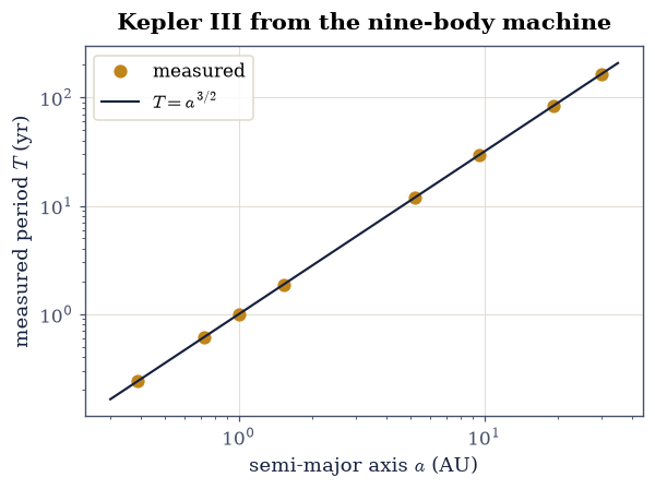
Fig. 108 Kepler’s third law recovered from the 350-year nine-body integration: each planet’s period, measured as \(2\pi\) over the fitted slope of its unwrapped heliocentric angle, against its semi-major axis on log–log axes. The fitted line has slope \(1.4989\); the planets’ sub-percent departures from it are real mutual perturbations, not measurement error.#
✓ every measured period meets T = a^(3/2)/√(1+m) at the percent level; the residuals are the mutual perturbations themselves [max|Δ| = 1.16054 (rtol=0.01, atol=1e-09)]
✓ the fitted log T–log a slope across all eight planets is Kepler's 3/2 [got 1.49895 vs expected 1.5 (rtol=0, atol=0.01)]
True
Exercise 4 — The long game: symplectic character versus accuracy#
§1.6 promised that the reason “molecular dynamics uses
velocity Verlet” would come due when integrations got long. Here it comes
due. We integrate the Sun–Earth–Jupiter three-body system (assembled by
the build_system you wrote in Exercise 2) for \(1000\) years two ways and
watch not the size of the energy error but its shape.
Part a) Velocity Verlet at \(\Delta t = 2\times10^{-3}\) yr
(\(5\times10^5\) steps). Record the relative energy error \(|E(t) - E_0|/|E_0|\)
every 500 steps. Verify it stays below \(10^{-7}\) for the entire millennium
and shows no trend: the mean error over the last hundred years
(numpy.mean over the sampled errors in each window) must be within a
factor of \(3\) of the mean over the first hundred (a wobble revisits its
floor; a drift does not).
Part b) Adaptive Runge–Kutta (scipy.integrate.solve_ivp, RK45,
rtol=1e-6, atol=1e-9, dense sampling every \(2\) yr) on the identical
system. Verify its final energy error exceeds Verlet’s maximum by a
factor above \(30\), and that its error grows monotonically in time (the
error at \(250\)-yr checkpoints strictly increasing): per step it is the
better integrator; per millennium it is the wrong one. The moral, plotted
in Fig. 109, is the deepest lesson this notebook has to
teach, and it travels far beyond gravity: the molecular-dynamics
simulations of Volume V’s horizon live and die by it.
Verlet max |ΔE/E| : 5.45e-08
Verlet early/late mean : 3.03e-08 / 2.99e-08
RK45 final |ΔE/E| : 8.15e-05
RK45 checkpoints : ['2.0e-05', '4.1e-05', '6.1e-05', '8.1e-05']
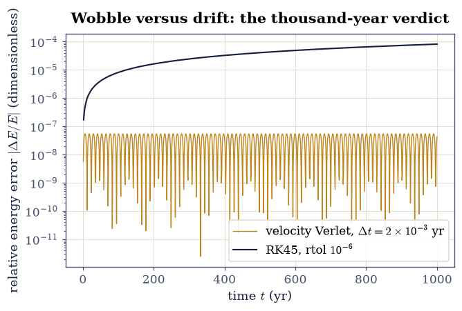
Fig. 109 One thousand years of the Sun–Earth–Jupiter system, integrated by symplectic velocity Verlet at fixed \(\Delta t=2\times10^{-3}\) yr (amber) and by adaptive RK45 at rtol \(10^{-6}\) (ink), on a logarithmic energy-error axis. Verlet’s error oscillates forever below \(10^{-7}\) with no secular trend; RK45’s per-step superiority is annihilated by one-signed accumulation, a drift that tolerance settings postpone but never remove.#
✓ the symplectic millennium: Verlet's energy error stays below 1e-7 and shows no secular trend (late mean within 3× the early mean) [max 5.4e-08, early 3.0e-08, late 3.0e-08]
✓ RK45's drift overwhelms Verlet's wobble by more than 30× at year 1000 [ratio 1496×]
✓ and the drift is secular: strictly increasing at every 250-year checkpoint — one-signed accumulation, not a wobble [checkpoints ['2.0e-05', '4.1e-05', '6.1e-05', '8.1e-05']]
True
Exercise 5 — A thought experiment: Jupiter at a thousand times the mass#
How fragile is the arrangement? The time-honoured numerical experiment (run in every computational-physics course since the machines could manage it) is brutal and illuminating: multiply Jupiter’s mass by \(1000\) — making it a \(0.955\,M_\odot\) companion star at \(5.2\) AU, and the Sun half of a binary — and watch what survives. The answer is not “nothing”: a planet deep inside a binary can orbit one star stably, and the boundary between safe and doomed has been mapped numerically, most famously by Holman and Wiegert [HW99], whose fitted critical semi-major axis for orbits around one star of a coplanar binary (mass fraction \(\mu\), eccentricity \(e_b\), separation \(a_b\)) is
their least-squares fit to a grid of long numerical integrations — an equation born from the kind of experiment this exercise runs. For our heavy Jupiter, \(\mu = 0.488\) and \(e_b = 0.049\) give \(a_c \approx 1.36\) AU: Earth at \(1.00\) AU should survive, and Mars at \(1.52\) AU should not.
Part a) Integrate Sun, Earth, Mars, and the normal Jupiter (the
system assembled, as always now, by your Exercise 2 build_system) with
verlet_orbits for \(50\) yr at \(\Delta t = 10^{-3}\) yr and record both
planets’ heliocentric distances.
Verify Earth stays within the narrow annulus \([0.97, 1.04]\) AU and Mars
within \([1.35, 1.70]\) AU (each planet’s eccentricity-driven excursion plus
Jupiter’s real, gentle nudging).
Part b) Rebuild the same system with \(m_{\rm Jup} \to 1000\,m_{\rm Jup}\) (the barycentric launch adjusts consistently) and integrate \(200\) yr at \(\Delta t = 5\times10^{-4}\) yr. Compute \(a_c\) from Eq. 133 and verify the two fates it predicts: Earth’s distance stays bounded within \([0.85, 1.15]\) AU — jostled, but bound — while Mars is ejected outright, its maximal heliocentric distance exceeding \(30\) AU (past Neptune’s orbit; in fact it leaves by thousands of AU). The stability boundary of the new binary runs between the two orbits, and the comparison figure tells the story: the ordinary solar system’s tameness is a property of its mass ratios, not of gravity.
real Jupiter : Earth in [0.9833, 1.0168] AU, Mars in [1.3812, 1.6662] AU
heavy Jupiter : a_c = 1.362 AU; Earth in [0.914, 1.099] AU; Mars r_max = 129261 AU
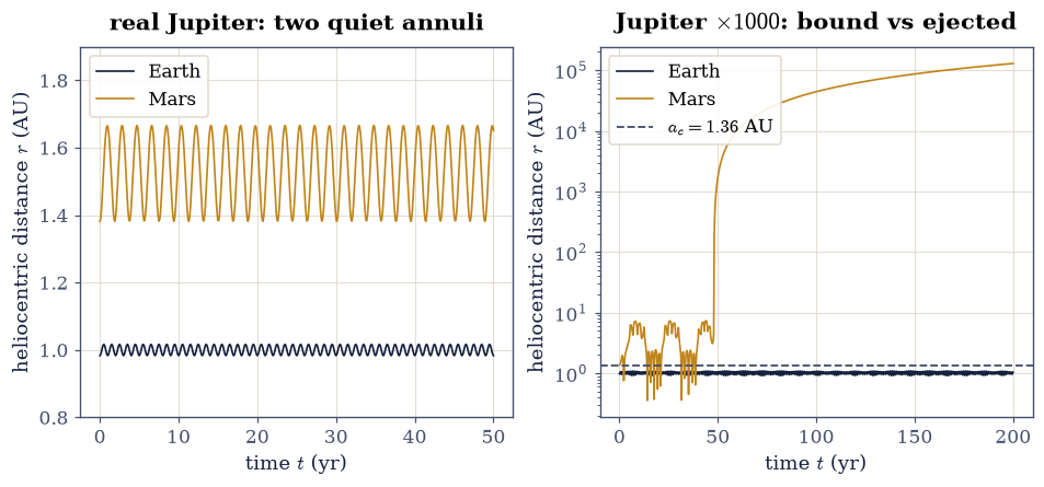
Fig. 110 Two fates, one stability boundary. Left: with the real Jupiter, fifty years confine Earth (ink) and Mars (amber) each to a narrow annulus set by its own eccentricity plus Jupiter’s gentle nudging. Right: with Jupiter’s mass multiplied by one thousand — a \(0.955\,M_\odot\) companion at \(5.2\) AU — Earth, inside the Holman–Wiegert critical radius \(a_c \approx 1.36\) AU (dashed), stays bound in a jostled but confined band, while Mars, outside it, is ejected from the system entirely (logarithmic axis: its distance climbs past Neptune within a century and keeps going).#
✓ with the real Jupiter, fifty years keep Earth inside [0.97, 1.04] AU and Mars inside [1.35, 1.70] AU [Earth [0.9833, 1.0168], Mars [1.3812, 1.6662]]
✓ the Holman–Wiegert critical radius of the new binary falls between the two orbits: a_c separates Earth from Mars [1.0 < a_c = 1.362 < 1.524 AU]
✓ Earth, inside a_c, survives two centuries beside a companion star: jostled but bound in [0.85, 1.15] AU [[0.914, 1.099]]
✓ Mars, outside a_c, is ejected: it leaves the planetary system past Neptune's orbit [r_max = 129261 AU]
True
Exercise 6 — The Galilean clockwork: the Laplace resonance#
Jupiter runs a solar system in miniature, and its three inner large moons keep the most famous appointment in celestial mechanics. Io, Europa, and Ganymede orbit with sidereal periods \(1.769138\), \(3.551181\), and \(7.154553\) days — near the ratio \(1\!:\!2\!:\!4\), but near is the wrong word: the pairwise ratios are \(2.0073\) and \(2.0147\), off from \(2\) in the third digit. The true lock, found by Laplace, is not in the pairs but in the combination of mean motions \(n_i = 2\pi/T_i\):
exact to observational precision (the associated resonance angle librates about \(180°\), so a triple conjunction of the three moons can never occur). The resonance has a thermal consequence worth the detour: by continually exchanging momentum at the same orbital phases, it holds Io and Europa on eccentric orbits that Jupiter’s tides would otherwise have circularized long ago. A moon on an eccentric orbit is kneaded — stretched and relaxed every orbit — and the dissipated work has to go somewhere: roughly \(100\) terawatts in Io, which makes it the most volcanically active body in the solar system, and enough in Europa to maintain a liquid-water ocean beneath its ice shell. Peale, Cassen, and Reynolds published the prediction that tides should melt Io [PCR79] three days before Voyager 1 arrived and photographed the volcanic plumes: one of the cleanest called shots in planetary science, and it begins with the arithmetic of Eq. 134.
Part a) The arithmetic. From the three quoted sidereal periods,
form the mean motions \(n_i = 2\pi/T_i\) and verify: the pairwise ratios
equal \(2.00729\) and \(2.01470\) (rtol=1e-4) — genuinely not \(2\) — while
the Laplace combination \(|n_{\rm Io} - 3n_{\rm Eu} + 2n_{\rm Ga}|/
n_{\rm Io}\) is below \(10^{-5}\): four orders of magnitude smaller than
the pairwise offsets. The resonance lives in the combination.
Part b) The measurement. Put the miniature system in the machine:
rebuild PLANETS (temporarily, restoring it afterwards as in Exercise
5) and hand the rebuilt table to your Exercise 2 build_system, with
Jupiter as the central mass and the three moons at their real
masses (in \(M_{\rm Jup}\): \(4.70\times10^{-5}\), \(2.53\times10^{-5}\),
\(7.81\times10^{-5}\)), semi-major axes (in units of \(10^6\) km: \(0.4217\),
\(0.6710\), \(1.0704\)), and eccentricities (\(0.0041\), \(0.0090\),
\(0.0013\)). With the central mass set to one, the unit system of
Eq. 130 works unchanged — \(G = 4\pi^2\) simply defines the
time unit. Integrate \(60\) Io orbits with verlet_orbits at \(\Delta t =
2\times10^{-4}\) (sampling every \(50\) steps keeps Io’s unwrapped angle
well under \(\pi\) per sample), measure the three mean motions with the
unwrap-and-fit of Exercise 3, and verify: the measured ratios match the
real ones to rtol=1e-3, and the measured Laplace combination stays
at least \(30\) times smaller than the smallest pairwise offset
\(|n_{\rm Io}/n_{\rm Eu} - 2|\). (Our launch does not phase-lock the
moons — that would require placing them at the librating configuration
— so the measured combination is small rather than zero; the point the
integration makes is that the near-cancellation is carried by the
orbits themselves, not by a numerical coincidence.)
The bar chart below is a still photograph of something that is really a statement about rates, so the player that follows it sets the same integrated system going. Watch the counters rather than the orbits: by the time Ganymede has come round once, Europa has come round twice and Io four times, and the three curves cross the dotted guides at \(1\), \(2\), and \(4\) together. That is the \(1\!:\!2\!:\!4\) of Eq. 134 seen from the other side, because periods in the ratio \(T_{\rm Io} : T_{\rm Eu} : T_{\rm Ga} = 1 : 2 : 4\) are revolutions accumulating in the reciprocal ratio \(4 : 2 : 1\). Nothing in the player is yours to build — the animation you wrote in Exercise 2 already covers that ground — but its physics is gated like everything else here.
ratios (real): 2.00729, 2.01470
ratios (meas): 2.00719, 2.01430
Laplace combination /n_Io: real 1.41e-07, measured 4.45e-05 (pair offset 7.19e-03)
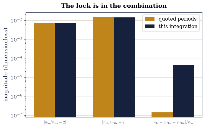
Fig. 111 The Laplace resonance ledger, on a logarithmic axis: the pairwise mean-motion offsets \(|n_{\rm Io}/n_{\rm Eu}-2|\) and \(|n_{\rm Eu}/n_{\rm Ga}-2|\) against the normalized Laplace combination \(|n_{\rm Io}-3n_{\rm Eu}+2n_{\rm Ga}|/n_{\rm Io}\), from the quoted sidereal periods (amber) and from this notebook’s own 60-orbit integration of the Jupiter–Io–Europa–Ganymede system (ink). The pairwise ratios miss the integers by nearly one percent; the combination cancels four to five orders of magnitude more deeply: the resonance is a property of the combination, not the pairs.#
✓ the quoted periods give pairwise ratios 2.00729 and 2.01470: genuinely not 2, at the third digit [max|Δ| = 4.51292e-06 (rtol=0.0001, atol=1e-09)]
✓ yet the Laplace combination n_Io - 3n_Eu + 2n_Ga cancels four orders more deeply than the pairwise offsets: eq-ss-laplace [|combo|/n_Io = 1.4e-07]
✓ the 60-orbit integration of the miniature system reproduces both real mean-motion ratios [max|Δ| = 0.000396942 (rtol=0.001, atol=1e-09)]
✓ and carries the same deep cancellation: the measured combination sits far below the pairwise offsets, without any phase-locking by hand [combo 4.4e-05 vs pair offset 7.2e-03]
True