3.10 Radiation

Elementary Computational Physics

Volume III — Classical Electrodynamics Notebook 3.10

What makes the waves: accelerating charges. Retarded potentials and causality, the oscillating dipole and its sin²θ pattern, the Larmor formula, and the ω⁴ law that explains why the sky is blue.

Level · advanced   •   Est. · 120–150 min

Raymond Amador v1.4.0  ·  2026-07-31  ·  CC BY 4.0 (text) / MIT (code)

Notebook overview

§3.8 proved that electromagnetic waves can exist; this one shows what makes them. The answer is sharp: accelerating charges radiate. A charge sitting still carries a static field, and a charge gliding at constant velocity carries its field along with it, but a charge that accelerates sheds a disturbance that detaches and travels to infinity. That shed disturbance is light, radio, and X-rays alike.

Two ideas organize the story. The first is causality through the retarded potentials: the field here and now depends on what the source was doing at the earlier time \(t_r=t-r/c\), because influence travels at \(c\). These retarded potentials are exactly the solutions of the Lorenz-gauge wave equations of §3.8, so they quietly close the gauge arc that began in §3.6: the gauge choice made there returns here as the causal, propagating field. The second idea is the \(1/r\) radiation field. Expanding the retarded field in powers of \(1/r\) gives near-field terms (\(1/r^2\), \(1/r^3\), the quasi-static fields of §3.1 and §3.5) and a single slowly-falling \(1/r\) term. Only that term carries energy to infinity, because its Poynting flux (\(\propto 1/r^2\)) times the sphere area (\(4\pi r^2\)) stays finite as \(r\to\infty\). Radiation is the \(1/r\) part.

From there everything follows: the oscillating dipole with its \(\sin^2\theta\) doughnut pattern, the total power \(P=\mu_0 p_0^2\omega^4/12\pi c\), the \(\omega^4\) law that makes blue light scatter twelve times more strongly than red (why the sky is blue), and the Larmor formula \(P=\mu_0 q^2 a^2/6\pi c\) for a single accelerating charge, whose corollary, that a classical orbiting electron must spiral into the nucleus, is one of the cracks that forced quantum mechanics.

Everything is in SI units, with \(c=1/\sqrt{\mu_0\varepsilon_0}\). A radiating field genuinely propagates, so exactly one figure here is animated, the dipole’s wavefronts detaching and travelling outward; everything else is a still.

How to read the checks. Each exercise ends with a validate call against an independent fact: an observed phase lag equal to \(\omega r/c\), a power through a sphere independent of its radius, the \(\sin^2\theta\) pattern integrating to \(8\pi/3\), the \(\omega^4\) ratio, the Larmor power. A ✓ is strong evidence; a ✗ is a prompt to locate the discrepancy, not a verdict.

Scope. A working review, not a full course. See Nolting, Theoretical Physics 3 [Nol16]; Griffiths, Introduction to Electrodynamics [Gri17] (ch. 11); Jackson [Jac98] (ch. 9, 14).

Theory in brief

Retarded potentials and causality

A change in the source cannot be felt instantly; it propagates at \(c\). The potentials at a field point therefore depend on the source at the retarded time \(t_r=t-r/c\),

(243)\[V(\mathbf r,t)=\frac{1}{4\pi\varepsilon_0}\int\frac{\rho(\mathbf r',t_r)}{|\mathbf r-\mathbf r'|}\,d^3r', \qquad t_r = t-\frac{|\mathbf r-\mathbf r'|}{c}.\]

These are precisely the solutions of the Lorenz-gauge wave equations \(\Box V=-\rho/ \varepsilon_0\), \(\Box\mathbf A=-\mu_0\mathbf J\) of §3.8, so the gauge choice made there yields the causal field here, closing the gauge arc; Griffiths, Introduction to Electrodynamics, ch. 10, verifies by direct differentiation that the retarded potentials do solve them. Causality is the new structural idea: the field knows only the source’s past.

Why acceleration radiates

A static charge has a static field; a uniformly moving charge carries its field rigidly along. Only an accelerating charge produces a field that detaches and propagates,

(244)\[\text{radiation} \iff \text{acceleration} \neq 0 .\]

A brief acceleration puts a transverse kink in the field lines that travels outward at \(c\), the radiation pulse.

The radiation field versus the near field

Expanding the retarded field in \(1/r\) gives near-field terms and one radiation term,

(245)\[\mathbf E = \underbrace{\mathcal{O}(1/r^2)+\mathcal{O}(1/r^3)}_{\text{near field}} + \underbrace{\mathcal{O}(1/r)}_{\text{radiation}} .\]

Only the \(1/r\) term carries net energy to infinity: its Poynting flux \(\propto 1/r^2\) times the sphere area \(4\pi r^2\) stays finite as \(r\to\infty\), while the near-field flux vanishes. Radiation is exactly the slowly-falling \(1/r\) part.

The oscillating dipole

For a dipole \(p(t)=p_0\cos\omega t\) the radiation field falls as \(1/r\) and has the angular power pattern

(246)\[\frac{dP}{d\Omega}\propto\sin^2\theta, \qquad P = \frac{\mu_0 p_0^2\omega^4}{12\pi c},\]

zero along the dipole axis and maximum broadside, the toroidal “doughnut”. Griffiths, Introduction to Electrodynamics, ch. 11, carries the retarded-potential computation behind both results out in full.

The \(\omega^4\) law

Radiated power scales as the fourth power of frequency,

(247)\[P \propto \omega^4 .\]

Air molecules driven by sunlight are little dipoles, so blue light (higher \(\omega\)) scatters about \((\nu_{\text{blue}}/\nu_{\text{red}})^4\approx12\) times more than red: why the sky is blue and sunsets red (Rayleigh scattering).

The Larmor formula

For a single point charge of acceleration \(a\),

(248)\[P = \frac{\mu_0 q^2 a^2}{6\pi c},\]

radiated power \(\propto a^2\). The dipole result is its oscillating-source special case; Jackson, Classical Electrodynamics, ch. 14, derives the general formula from the fields of an arbitrarily moving point charge.

Setup

Data and instruments only: the SI constants (\(\mu_0\), \(\varepsilon_0\), and the speed of light built from them), the series palette, the three closed-form radiation laws this notebook is about rather than builds — the \(\sin^2\theta\) pattern, the dipole power \(\mu_0p_0^2\omega^4/12\pi c\), and the Larmor power \(\mu_0q^2a^2/6\pi c\), each a one-line transcription of an equation displayed above — and the far-field slice that the wavefront animation of Exercise 4 paints. The measuring is not here: the retarded-phase fit of Exercise 1, the solid-angle quadratures of Exercises 3, 5 and 8, and the \(\omega^4\) ratio of Exercise 6 are all built in their exercises. No randomness appears anywhere in this notebook.

The Setup below holds this notebook’s data and instruments — nothing you are asked to build. It is collapsed so the building stays yours; expand it whenever you want the details.

Show code cell source

Hide code cell source

import numpy as np
import matplotlib.pyplot as plt
from matplotlib.animation import FuncAnimation

from ecp import draw, validate
from ecp.animate import show

from scipy.constants import mu_0 as MU0  # data: vacuum permeability, T·m/A
from scipy.constants import epsilon_0 as EPS0  # data: vacuum permittivity, F/m

C_LIGHT = 1.0 / np.sqrt(MU0 * EPS0)  # data: speed of light c = 1/√(μ0ε0), m/s
ACCENT, INK, SOFT = draw.ACCENT, draw.INK, draw.SOFT  # data: the series palette


# data: the dipole's angular pattern exactly as eq-dipole-radiation displays it —
# sin²θ, with nothing to construct beyond the equation itself. It is the specimen
# Exercise 4 measures (null on axis, peak broadside, integral 8π/3), not machinery.
def dipole_power_pattern(theta):
    """Angular radiation pattern dP/dΩ ∝ sin^2 θ of a dipole (eq-dipole-radiation).

    The normalised pattern of an oscillating electric dipole: it vanishes along
    the axis (θ = 0, π) and peaks broadside (θ = π/2), the cross-section of the
    toroidal "doughnut".

    Parameters
    ----------
    theta : float or numpy.ndarray
        Polar angle from the dipole axis, in radians.

    Returns
    -------
    float or numpy.ndarray
        The relative power per solid angle, sin^2 θ.
    """
    return np.sin(theta) ** 2


# data: the closed form of eq-dipole-radiation, transcribed. The deriving happens on
# paper (Griffiths ch. 11); Exercises 5 and 6 measure a quadrature against it and take
# a frequency ratio through it, so it is the given answer, not the notebook's method.
def dipole_total_power(p0, omega):
    """Total time-averaged power radiated by an oscillating dipole (eq-dipole-radiation).

    P = μ0·p0^2·ω^4/(12π c): the ω^4 dependence is what makes high-frequency
    sources radiate so much more strongly.

    Parameters
    ----------
    p0 : float
        Dipole-moment amplitude, in C·m.
    omega : float
        Angular frequency, in rad/s.

    Returns
    -------
    float
        The total radiated power, in watts.
    """
    return MU0 * p0**2 * omega**4 / (12.0 * np.pi * C_LIGHT)


# data: the Larmor formula eq-larmor, transcribed. What Exercise 7 builds is the
# classical hydrogen orbit and its collapse time; evaluating this one-line law is the
# given input to that estimate.
def larmor_power(q, a):
    """Larmor power radiated by a single accelerating point charge (eq-larmor).

    P = μ0·q^2·a^2/(6π c), proportional to the square of the acceleration: the
    general statement of which the dipole formula is the oscillating-source
    case.

    Parameters
    ----------
    q : float
        Charge, in coulombs.
    a : float
        Acceleration magnitude, in m/s².

    Returns
    -------
    float
        The instantaneous radiated power, in watts.
    """
    return MU0 * q**2 * a**2 / (6.0 * np.pi * C_LIGHT)


# instrument: the picture-making scaffold for the one animation — the far field
# E ∝ sinθ·cos(ω(t−r/c))/r sampled on a plane grid, with the 1/r core masked so the
# colour scale survives the singularity. Nothing is measured against it (the physics it
# shows is certified numerically in Exercises 1 and 4), and the notebook would teach the
# same lesson had the animation arrived from a library.
def radiation_field_plane(X, Z, t, omega, eps=0.04):
    """Dipole radiation field in the x–z plane, for the propagation animation.

    The far-field form E ∝ sin θ · cos(ω(t − r/c))/r on a slice containing the
    dipole axis ẑ: outgoing wavefronts modulated by the sin θ pattern,
    brightest broadside and null along the axis. A small core radius ``eps``
    is masked to avoid the 1/r singularity at the source.

    Parameters
    ----------
    X, Z : numpy.ndarray
        Coordinate grids in the plane (z is the dipole axis).
    t : float
        Time at which to evaluate.
    omega : float
        Angular frequency, in rad/s.
    eps : float, optional
        Core radius masked near the origin (default 0.04).

    Returns
    -------
    numpy.ndarray
        The (arbitrary-amplitude) radiation field on the grid, with the core set to zero.
    """
    r = np.hypot(X, Z)
    sin_theta = np.abs(X) / np.where(r > 0, r, 1.0)
    k = omega / C_LIGHT
    field = np.where(
        r > eps, sin_theta * np.cos(omega * t - k * r) / np.maximum(r, eps), 0.0
    )
    return field

Exercise 1 — Retarded time and causality (worked)

Nothing the source does is felt instantly; its influence spreads at \(c\). The field at distance \(r\) at time \(t\) reflects the source at the retarded time \(t_r=t-r/c\) Eq. 243, so a harmonic source \(\cos(\omega t)\) is observed delayed, with a phase lag \(\omega r/c\) (Fig. 271). For a \(1\,\)GHz source at \(r=0.5\,\)m the delay is about \(1.7\,\)ns. These retarded potentials are exactly the Lorenz-gauge solutions of the §3.8 wave equations, so the gauge arc of §3.6–§3.8 closes here: the field carries only the source’s past.

1. Build the observed signal as the source \(\cos\omega t\) evaluated at the retarded time \(t_r=t-r/c\), sampled over twenty whole periods at \(f=1\,\)GHz and \(r=0.5\,\)m.

2. Measure its phase by projecting onto \(\cos\omega t\) and \(\sin\omega t\) — a least-squares phase fit, which over whole periods is exact — and confirm the lag it returns is \(\omega r/c\) modulo \(2\pi\).

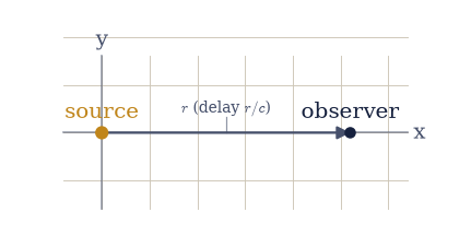
Fig. 271 Retardation: a source at the origin and an observer a distance \(r\) away on a coordinate grid. A change made now reaches the observer only after the light-travel time \(r/c\), so the observed field is the source evaluated at the earlier retarded time \(t_r=t-r/c\), lagging in phase by \(\omega r/c\). The field knows only the source’s past.

light-travel delay r/c = 1.668 ns
measured phase lag = 4.196040 rad,  ωr/c (mod 2π) = 4.196040 rad

Validation 1

✓  the observed field lags by ωr/c — the retarded-time delay (Lorenz-gauge solution)   [got 4.19604 vs expected 4.19604 (rtol=1e-06, atol=1e-09)]

True

Exercise 2 — Why acceleration radiates (worked)

Three charges, three different fates for their fields Eq. 244. A static charge has the radial \(1/r^2\) Coulomb field of §3.1, frozen in place. A charge in uniform motion carries that field rigidly along, with no piece left behind. Only an accelerating charge launches a disturbance that separates from it: a brief acceleration kinks the field lines, and the kink, the transverse \(1/r\) radiation field, races outward at \(c\) (Fig. 272).

The criterion is quantitative: the radiation-field amplitude is \(E_{\mathrm{rad}}\propto q\,a\,\sin\theta/(4\pi\varepsilon_0 c^2 r)\), linear in the acceleration \(a\) and in nothing else. The charge below is an electron, observed broadside (\(\theta=\pi/2\), where the pattern peaks) at \(r=1\,\)m.

1. Evaluate that closed-form amplitude at \(a=0\) (static or uniform motion) and at \(a\neq0\), and confirm the \(1/r\) term exists only when the charge accelerates.

2. Confirm the linearity property \(E_{\mathrm{rad}}(2a)=2\,E_{\mathrm{rad}}(a)\) — doubling the acceleration doubles the radiated field.

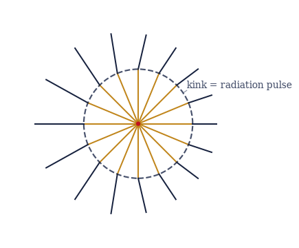
Fig. 272 The field-line kink of a briefly accelerated charge. Inside the shell \(r<ct\) (dashed) the lines point from the charge’s new position; outside they still point from where it used to be; across the shell they join in a transverse kink. That kink is the radiation pulse, the \(1/r\) field, sweeping outward at \(c\). A charge that never accelerated would have straight, unbroken radial lines and radiate nothing.

radiation field, a = 0     : 0.000e+00 V/m  (no 1/r term)
radiation field, a = 1e22  : 1.602e-04 V/m  (1/r term present)
E_rad(2a) = 2 E_rad(a): True  (linear in the acceleration)

Validation 2

✓  radiation requires acceleration: the 1/r far field appears only when a ≠ 0, and doubles when a doubles

True

Exercise 3 — Near field versus radiation field: the \(1/r\) point (worked)

This is the heart of radiation. The retarded field of an oscillating dipole splits into near-field pieces (\(\propto 1/r^2\) and \(1/r^3\), the quasi-static dipole field of §3.5) and a radiation piece (\(\propto 1/r\)) Eq. 245. The distinction is not cosmetic: the time-averaged Poynting flux of the radiation field falls as \(1/r^2\), so the power crossing a sphere, flux times \(4\pi r^2\), is independent of \(r\), while the near-field flux falls faster and carries nothing to infinity. Radiation is the slowly-falling \(1/r\) part, and that is exactly what lets energy escape.

The radiation field’s time-averaged flux is \(\langle S\rangle=\mu_0 p_0^2 \omega^4\sin^2\theta/(32\pi^2 c\,r^2)\); the dipole used here and in Exercise 5 has amplitude \(p_0=1\,\)nC·m and frequency \(f=1\,\)GHz.

1. Integrate the power through spheres of radius \(r=1\), \(10\), and \(100\,\)m (numpy.trapezoid over \(\theta,\varphi\) with the \(\sin\theta\) measure) and confirm it is the same number at every radius.

2. Contrast the near field, whose flux falls as \(1/r^4\) so its power through the sphere collapses as \(1/r^2\) (Fig. 273).

  r =      1 m:  radiation power = 1.732916e+05 W   near-field power ∝ 1e+00
  r =     10 m:  radiation power = 1.732916e+05 W   near-field power ∝ 1e-02
  r =    100 m:  radiation power = 1.732916e+05 W   near-field power ∝ 1e-04
analytic P = μ₀p₀²ω⁴/12πc = 1.732916e+05 W

Validation 3

✓  only the 1/r radiation field carries constant power to infinity (r-independent)   [max|Δ| = 2.91038e-11 (rtol=0.001, atol=1e-09)]

True

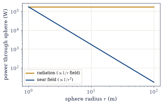
Fig. 273 Power crossing a sphere against its radius, for the radiation field (\(\propto 1/r\), amber) and a near-field term (\(\propto 1/r^2\), blue). The radiation power is flat: its flux \(\propto 1/r^2\) exactly cancels the \(4\pi r^2\) area, so the same energy crosses every sphere out to infinity. The near-field power collapses, carrying nothing away. Radiation is precisely the part that survives this limit.

Exercise 4 — The oscillating dipole and its \(\sin^2\theta\) pattern (worked)

The prototypical radiator is an oscillating electric dipole \(p(t)=p_0\cos\omega t\), an antenna in miniature. Its far field falls as \(1/r\) and carries the angular power pattern \(dP/d\Omega\propto\sin^2\theta\) Eq. 246: nothing radiates along the dipole axis, everything broadside, giving the toroidal doughnut (Fig. 274, Fig. 275). Integrated over solid angle the pattern gives \(\int\sin^2\theta\,d\Omega=8\pi/3\), the constant that Exercise 5’s total power and Exercise 8’s directivity both rest on.

The animation (Fig. 276) sets the same pattern in motion: the dipole’s wavefronts detach and travel outward at \(c\), brightest at the equator and dark along the poles, the iconic image of radiation.

1. Evaluate the pattern and confirm it vanishes along the axis (\(\theta=0\)) and peaks broadside (\(\theta=\pi/2\)).

2. Integrate it over the sphere with numpy.trapezoid (the \(\sin\theta\) measure) and confirm the result is \(8\pi/3\).

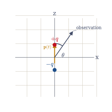
Fig. 274 An oscillating dipole \(p(t)=p_0\cos\omega t\) along the \(z\)-axis (red \(\pm\) charges, amber moment), with the observation direction at polar angle \(\theta\). The radiated power per solid angle is \(\propto\sin^2\theta\): zero along the axis (\(\theta=0\)) and maximum broadside (\(\theta=\pi/2\)), so the pattern is a torus wrapped around the dipole.

pattern on axis (θ=0): 0.000,  broadside (θ=π/2): 1.000
∫ sin²θ dΩ = 8.37758   (8π/3 = 8.37758)

Validation 4

✓  the sin²θ pattern integrates to 8π/3 over solid angle   [got 8.37758 vs expected 8.37758 (rtol=0.001, atol=1e-09)]
✓  the dipole pattern is null along the axis and maximal broadside

True

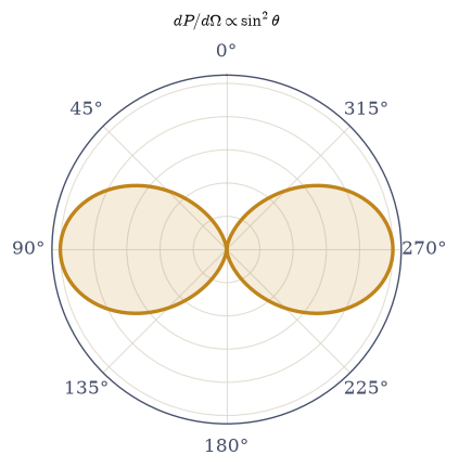
Fig. 275 The dipole radiation pattern \(dP/d\Omega\propto\sin^2\theta\) as a polar plot in a plane containing the axis (vertical). The two lobes are the cross-section of the toroidal doughnut: the radiation is strongest broadside and pinches to zero along the dipole axis (top and bottom). An antenna sends no power straight off its own ends.

Once Loop Reflect

Fig. 276 Animation of the radiating dipole: the far field \(E\propto\sin\theta\,\cos(\omega(t-r/c))/r\) in a plane containing the axis (vertical). Wavefronts (rings of one colour) form near the dipole, detach, and travel outward at \(c\), one free-space wavelength \(\lambda=2\pi c/\omega\) between like-coloured rings. They are brightest broadside (left–right) and vanish along the axis (top–bottom), the \(\sin\theta\) doughnut set into motion. This is radiation: energy leaving the source and never returning.

Exercise 5 — Total radiated power (worked)

Integrating the pattern over all directions gives the total power the dipole sheds. With the radiation intensity \(\langle S\rangle=\mu_0 p_0^2\omega^4\sin^2\theta/ (32\pi^2 c\,r^2)\), the angular integral \(\int\sin^2\theta\,d\Omega=8\pi/3\) of Exercise 4 collapses the constant and leaves \(P=\mu_0 p_0^2\omega^4/12\pi c\) Eq. 246. The dipole is the one of Exercise 3, \(p_0=1\,\)nC·m at \(f=1\,\)GHz, and the sphere is evaluated at \(r=1\,\)m — the answer cannot depend on that choice, which is what Exercise 3 established.

1. Integrate the intensity over solid angle with numpy.trapezoid (the \(r^2\sin\theta\) Jacobian), so that the angular distribution and the total power close one loop.

2. Confirm the result matches the closed form \(\mu_0 p_0^2\omega^4/12\pi c\), evaluated through the Setup’s dipole_total_power.

P (integrated)            = 1.732916e+05 W
P = μ₀p₀²ω⁴/12πc (closed)  = 1.732916e+05 W

Validation 5

✓  the total radiated dipole power is μ₀p₀²ω⁴/12πc   [got 173292 vs expected 173292 (rtol=0.01, atol=1e-09)]

True

Exercise 6 — The \(\omega^4\) law and why the sky is blue (student)

The steepest consequence of \(P\propto\omega^4\) Eq. 247 is overhead every clear day. Air molecules driven by sunlight act as tiny dipoles, re-radiating (scattering) the light that drives them, and with power \(\propto\omega^4\) the blue end of the spectrum scatters far more than the red. The ratio for blue (\(\lambda\approx400\,\)nm) over red (\(\lambda\approx750\,\)nm) is \((\nu_{\text{blue}}/\nu_{\text{red}})^4\) (Fig. 277).

Taking that ratio through the implemented power formula, rather than restating \((\nu_{\text{blue}}/\nu_{\text{red}})^4\) and comparing it with itself, is what makes the check bite: it is the code’s frequency scaling that is under test.

1. Compute the scattered-power ratio at blue against red optical frequencies with the Setup’s dipole_total_power, at fixed dipole amplitude.

2. Confirm it reproduces \((\nu_{\text{blue}}/\nu_{\text{red}})^4\) — the factor of about twelve that paints the daytime sky blue and the setting sun red.

ν_blue = 749.5 THz,  ν_red = 399.7 THz
P_blue / P_red (via dipole_total_power) = 12.36
(ν_b/ν_r)⁴                               = 12.36
blue scatters ~12× more than red: blue sky overhead, red light at sunset

Validation 6

✓  the implemented dipole power scales as ω⁴ (blue/red through the formula)   [got 12.3596 vs expected 12.3596 (rtol=1e-09, atol=1e-09)]
✓  the blue/red scattering ratio is the famous factor of about twelve   [P_blue/P_red = 12.36]

True

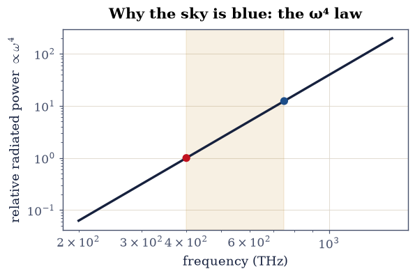
Fig. 277 Radiated (scattered) power against frequency on log axes, the steep \(P\propto\omega^4\) rise, with the visible band shaded from red to blue. Across the optical range the curve climbs by about a factor of twelve, so molecular scattering of sunlight is dominated by the blue end. The same \(\omega^4\) law makes shorter wavelengths the ones that get scattered out of a sightline first.

Exercise 7 — The Larmor formula and the classical-atom catastrophe (student)

The dipole result is one case of a more general law. Any single point charge of acceleration \(a\) radiates power \(P=\mu_0 q^2 a^2/6\pi c\) Eq. 248, the Larmor formula, depending only on the square of the acceleration. Its most famous corollary is a disaster for classical physics: an electron orbiting a proton is accelerating centripetally, so it must radiate, lose energy, and spiral into the nucleus.

The orbit to put through the formula is the classical hydrogen ground state, radius \(a_0=5.29\times10^{-11}\,\)m, where the Coulomb attraction supplies the centripetal force and the orbit’s binding energy is \(|E|=k_e e^2/2a_0\). A classical atom would collapse in a fraction of a nanosecond. That it does not is one of the cracks, alongside the “speed relative to what?” of §3.8, through which quantum mechanics enters (Vol VI).

1. Compute the centripetal acceleration \(a=k_e e^2/(m_e a_0^2)\) and the Larmor power the electron radiates at it.

2. Estimate the collapse time as the orbit’s energy divided by that power — an order-of-magnitude figure, since the power grows as the orbit shrinks.

centripetal acceleration = 9.044e+22 m/s²
Larmor power = 4.669e-08 W
order-of-magnitude collapse time ≈ 46.685 ps

Validation 7

✓  Larmor: radiated power ∝ acceleration²   [got 4.66929e-08 vs expected 4.66929e-08 (rtol=1e-06, atol=1e-09)]

True

Exercise 8 — Antennas and the reach of radiation

The dipole pattern is the foundation of antenna theory. Its directivity measures how focused the radiation is: the peak intensity divided by the average over all directions, \(D=4\pi(dP/d\Omega)_{\max}/P\). For the ideal dipole, \(\sin^2\theta\) peaks at 1 and integrates to \(8\pi/3\), so \(D=3/2\), a modest but real concentration broadside. From this seed grow phased arrays, dish feeds, and the directional antennas that carry signals across the planet and beyond, all the same retarded-field physics that carries starlight to a telescope. From a wiggling charge to a signal across the galaxy: §3.8 showed waves can exist, and this notebook showed what makes them, completing the volume’s wave story.

1. Form the pattern’s solid-angle average from the \(\int\sin^2\theta\,d\Omega\) you integrated in Exercise 4, and divide the broadside peak by it.

2. Confirm the directivity is \(3/2\).

⟨pattern⟩ over the sphere = 0.6667
directivity D = peak/average = 1.5000   (ideal dipole 3/2 = 1.5)

Validation 8

✓  the ideal dipole directivity is 3/2   [got 1.5 vs expected 1.5 (rtol=0.001, atol=1e-09)]

True

Notebook summary

• Causality through retarded potentials Eq. 243: the field carries the source’s past, observed with a phase lag \(\omega r/c\) (verified to \(10^{-6}\)). These are the Lorenz-gauge solutions of the §3.8 wave equations, closing the gauge arc.

• Radiation requires acceleration Eq. 244: the \(1/r\) far field is linear in \(a\) and vanishes for a static or uniformly moving charge; a brief acceleration kinks the field lines and the kink propagates at \(c\).

• The \(1/r\) point Eq. 245: only the radiation field carries constant power through spheres of every radius (verified \(r\)-independent), while the near field’s flux collapses. Radiation is the slowly-falling \(1/r\) part.

• The oscillating dipole Eq. 246: the \(\sin^2\theta\) doughnut (null on axis, peak broadside) integrates to \(8\pi/3\), giving \(P=\mu_0 p_0^2\omega^4/ 12\pi c\); the wavefronts were animated detaching and travelling outward.

• The \(\omega^4\) law Eq. 247: blue scatters \(\approx12\times\) more than red, why the sky is blue; the Larmor power Eq. 248 \(\propto a^2\) implies a classical atom would collapse in picoseconds; and the ideal-dipole directivity is \(3/2\), the seed of antenna theory.

Outlook

• Antenna engineering. Arrays and beam-forming sharpen the modest \(D=3/2\) into highly directional beams; the half-wave dipole is the practical workhorse.

• Radiation from charges in fields. Synchrotron radiation (circular motion) and bremsstrahlung (deceleration) are Larmor radiation in disguise, the light sources of modern X-ray science.

• The radiation reaction. A radiating charge must recoil from the momentum it sheds; the resulting self-force is a famously subtle corner of classical electrodynamics.

• The classical-atom catastrophe (Vol VI). That the Larmor collapse does not happen is a direct route into quantum mechanics.

• The relativistic capstone (§3.12). Radiation, the retarded potentials, and the \(\mathbf E\)/\(\mathbf B\) split are most naturally written in covariant form, where the “speed relative to what?” of §3.8 is finally answered.

Take this notebook with you

Use the download button (↓) in the toolbar above to save this notebook and run it yourself. The published notebooks ship without worked solutions; if you would like the reference solutions — to teach from or to check your own work — get in touch: hello@ramador.me.