1.7 The Falling Chain

Elementary Computational Physics

Volume I — Elementary Mechanics Notebook 1.7

Three chains, three surprises: a chain pouring off a table, a chain piling on the floor with three times its weight, and a folded chain that falls faster than gravity. Variable-mass mechanics and where energy quietly disappears.

Level · advanced   •   Est. · 90–120 min

Raymond Amador v1.4.0  ·  2026-07-31  ·  CC BY 4.0 (text) / MIT (code)

Notebook overview

A chain is the simplest system in which mass is set into motion (or stopped) a bit at a time, and that single complication overturns the reflex that “it’s just gravity.” We take one idealised chain (inextensible, perfectly flexible, linear density \(\lambda\)) through three classic situations, and in each the naive answer is wrong in a different way:

1. Act I: a chain sliding off a table. The gentle case: nothing changes speed abruptly, energy is conserved, and the overhang grows like \(\cosh\).

2. Act II: a chain piling on the floor. Landing links must be stopped, and the floor reads three times the weight already landed.

3. Act III: a folded chain, one end released. The subtle case: the free end falls faster than \(g\), and the two textbook analyses (energy versus momentum) disagree about where the energy goes.

The unifying tool is Newton’s law in its general form, \(\mathbf F_\text{ext} = d\mathbf p/dt\) for the whole system, applied with care to the momentum carried by mass entering or leaving the moving part. This is the classical cousin of the rocket equation, and most “chain paradoxes” are just \(F=ma\) used where it does not apply.

How to read the checks. Each exercise ends with a validate call against an independent fact: a closed-form solution, a conserved quantity, an exact ratio. A ✓ is strong evidence we got it right; a ✗ is a prompt to locate the discrepancy (a sign, a missing momentum-flux term, too tight a tolerance), not a verdict.

Scope. A working review, not a treatise on variable-mass dynamics. For the underlying mechanics see Nolting, Theoretische Physik 1 [Nol16]; the chain problems are Cambridge/Irodov staples, and the folded chain in particular has a careful modern literature (Calkin & March) that we follow.

Theory in brief

Newton’s law when the moving mass changes

For a body of fixed mass, \(F=ma\). When mass is continuously added to or removed from the moving part, that is no longer the right statement; the safe law is Newton’s original one, applied to a fixed collection of matter (a closed system):

(123)\[\mathbf F_\text{ext} = \frac{d\mathbf p}{dt},\]

where \(\mathbf p\) is the total momentum of all the matter and \(\mathbf F_\text{ext}\) the total external force. The trap is to write \(F = \frac{d}{dt}(mv) = \dot m v + m\dot v\) for the moving piece alone and forget that the mass crossing the boundary also carries momentum. Done correctly (accounting for the momentum flux of the mass entering or leaving) Eq. 123 is unambiguous. (Each act below applies it to its own boundary.)

Energy is not guaranteed

Momentum/force bookkeeping is always valid. Energy conservation is not. When a link is jerked from rest to speed \(v\) (or from \(v\) to rest) over an infinitesimal distance, that is an inelastic event (like a perfectly inelastic collision), and mechanical energy can be lost to it:

(124)\[\frac{dE_\text{mech}}{dt} \le 0 \quad\text{when links change speed abruptly.}\]

So the reliable strategy is always force/momentum first; then ask, separately, whether energy happened to be conserved. Act I conserves it (nothing jerks); Act II plainly dissipates it (links slam to rest); Act III is the subtle one, where the answer depends on how the chain negotiates its fold, and that is the whole lesson. The per-act theory is developed in each act’s statement below.

Setup

Data and instruments only — this notebook’s Setup defines no functions at all. It holds NumPy and Matplotlib, the two SciPy routines the acts lean on (solve_ivp for the equations of motion, minimize_scalar for the staging optimum), the ecp diagram, validation and animation helpers, and the three numbers that fix the idealised chain: its linear density \(\lambda\), its length \(L\), and \(g\). Every equation of motion the notebook is about — the table chain’s \(\ddot x = (g/L)x\), the floor’s momentum-flux bookkeeping, the folded chain’s \(v^2(x)\) and \(a(x)\), and the rocket’s variable-mass integrand — you write in the act that calls for it.

The Setup below holds this notebook’s data and instruments — nothing you are asked to build. It is collapsed so the building stays yours; expand it whenever you want the details.

Show code cell source

Hide code cell source

import numpy as np
import matplotlib.pyplot as plt
from scipy.integrate import solve_ivp
from scipy.optimize import minimize_scalar

from ecp import draw, validate
from ecp.animate import show

# data: the idealised chain — inextensible, perfectly flexible, uniform.
LAM = 1.0  # linear mass density  λ  [kg/m]
L = 1.0  # chain length  L  [m]
G = 9.81  # gravitational acceleration  g  [m/s²]

---

Act I — A chain sliding off a table edge

The setup and its theory. A uniform chain of length \(L\) and linear density \(\lambda\) lies on a frictionless table; a short piece of length \(x\) hangs over the edge (Fig. 99). Only the hanging piece feels a net pull (its weight \(\lambda x g\)), but it drags the whole chain of mass \(\lambda L\) with it (the chain is inextensible, so every link moves at the same speed \(\dot x\)). No link changes speed abruptly here, so Eq. 123 reduces to ordinary \(F=ma\) on the whole chain:

(125)\[(\lambda L)\,\ddot x = (\lambda x)\,g \qquad\Longrightarrow\qquad \ddot x = \frac{g}{L}\,x, \qquad 0 < x < L.\]

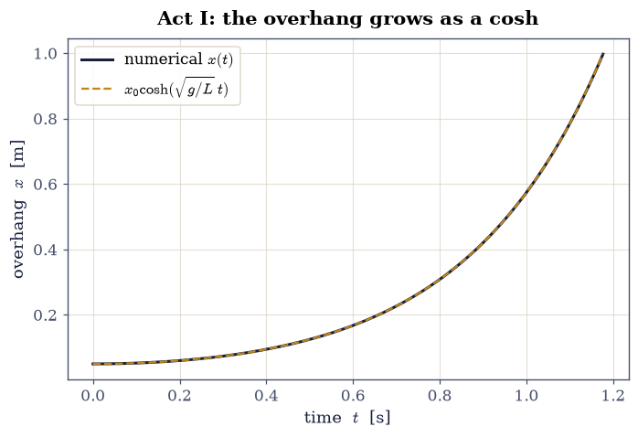
This is the unstable linear equation \(\ddot x = +\omega^2 x\) with \(\omega=\sqrt{g/L}\) (exponential growth, not oscillation), so from rest at \(x_0\) it solves to \(x(t) = x_0\cosh(\sqrt{g/L}\,t)\). Because nothing is jerked, energy is conserved; this is the calibration case where energy and momentum agree, and it comes with a closed form and a conserved quantity to check against.

1. Write table_rhs(t, s), the state derivative of Eq. 125 for the state \(s=(x,\dot x)\), and a terminal leave_table event that fires when the last link leaves the table. Write this one yourself — turning the force balance into a state derivative is the lesson.

2. Integrate it from a small overhang with scipy.integrate.solve_ivp (default RK45, rtol=1e-11, atol=1e-12, dense t_eval) and plot \(x(t)\).

3. Compare to the closed form \(x_0\cosh(\sqrt{g/L}\,t)\).

4. Evaluate the total energy \(E=\tfrac12\lambda L\dot x^2-\tfrac12\lambda g x^2\) along the solution and confirm its relative drift stays at the solver tolerance: energy is conserved while the chain slides.

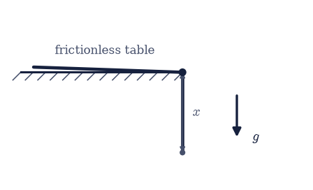
Fig. 99 A uniform chain on a frictionless table with a length \(x\) hanging over the edge (marked point): the overhang’s weight \(\lambda x g\) drives the whole chain of mass \(\lambda L\), with \(g\) the gravitational acceleration. No link changes speed abruptly, so energy is conserved while the chain slides.

Solution — Act I

Validation — Act I

✓  the table chain follows x₀cosh(√(g/L)t)   [max|Δ| = 1.15767e-11 (rtol=1e-06, atol=1e-09)]
✓  energy is conserved while the chain slides (no dissipation)   [max relative drift = 2.00864e-11 (limit 1e-06)]

True

---

Act II — A chain falling onto the floor

The setup and its theory. Now hold the chain vertically with its lower end just touching a floor (or scale) and release it (Fig. 100). The chain falls freely; as it does, its bottom links reach the floor and stop dead. What does the floor read when a length \(y\) has piled up?

Apply Eq. 123 to the floor’s contact force. It has two parts. First, the static weight of the chain already at rest on the floor, \(\lambda y g\). Second, the force to stop the arriving links: in a time \(dt\) a length \(v\,dt\) lands, i.e. mass \(dm = \lambda v\,dt\) arriving at speed \(v\), so the floor must destroy momentum at the rate \(\dfrac{dm}{dt}\,v = \lambda v^2\). The links arrive in free fall, \(v^2 = 2gy\), hence

(126)\[F = \underbrace{\lambda y g}_{\text{weight landed}} + \underbrace{\lambda v^2}_{\text{stopping force}} = \lambda y g + 2\lambda y g = 3\,\lambda y g,\]

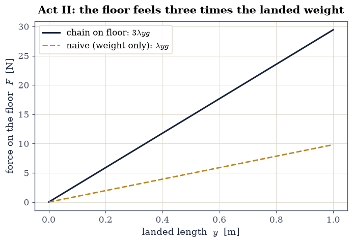
three times the weight of the chain on the floor. Stopping mass is not free. The factor of three is exact and independent of \(y\), so it holds throughout the fall, and the naive expectation it corrects is the landed weight \(\lambda y g\) alone.

1. Implement the two contributions and the total \(F(y)\) on a grid of landed lengths (numpy.linspace).

2. Show the ratio \(F/(\lambda y g)\) equals exactly \(3\) throughout the fall.

3. Plot the force against the naive expectation (just the landed weight).

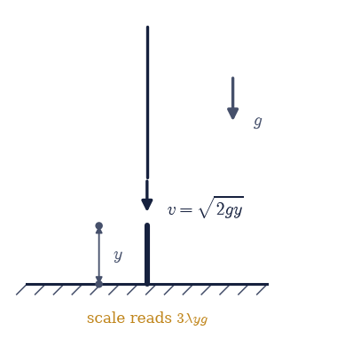
Fig. 100 A chain released from rest falling onto a scale: a length \(y\) has piled up (the landed chain, marked), arriving links land at speed \(v=\sqrt{2gy}\) and are stopped. The scale reads \(F=3\lambda y g\) — the static weight \(\lambda y g\) of the pile plus the momentum-stopping force \(\lambda v^2 = 2\lambda y g\).

Solution — Act II

mean F/(λyg) = 3.000000

We caption the comparison as a numbered figure, since it carries the headline factor-of-three result.

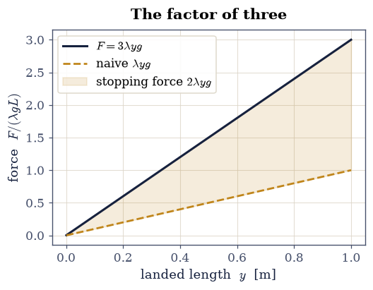
Fig. 101 Force on the floor versus the landed length \(y\) for a chain falling from rest: the full momentum bookkeeping (dark) gives \(3\lambda y g\), exactly three times the naive landed-weight expectation \(\lambda y g\) (dashed) — the extra \(2\lambda y g\) is the force needed to stop the arriving links.

Validation — Act II

✓  the floor force is three times the landed weight   [max|Δ| = 4.44089e-16 (rtol=1e-06, atol=1e-09)]

True

---

Act III — The folded falling chain

The setup and its theory (the subtle one). Fold the chain in two and hang it from the ceiling: one end is fixed, the other (the free end) starts beside it at the top and is released (Fig. 102). As the free end falls a distance \(x\), links peel off the moving strand and join the hanging strand at the fold. Geometry: with both strands measured from the ceiling, the fold sits at depth \((L+x)/2\), so the moving strand has length \((L-x)/2\) and shrinks as \(x\) grows.

Here the two textbook analyses disagree, and that disagreement is the point.

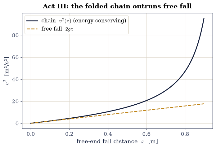
Energy-conserving chain. If the fold is an ideal frictionless bend that does no net work destroying motion (the modern, experimentally supported picture, Calkin & March), mechanical energy is conserved. Working out \(T+V=\text{const}\) for the shrinking moving strand gives the free-end speed

(127)\[v^2(x) = \frac{g\,x\,(2L - x)}{L - x}, \qquad a(x) = \tfrac12\frac{dv^2}{dx} = \frac{g\,(2L^2 - 2Lx + x^2)}{2\,(L-x)^2}.\]

Since \(v^2(x) > 2gx\) for all \(x>0\), the free end falls faster than free fall, and \(a(x) \ge g\) rising to \(\infty\) as \(x\to L\).

Inelastic-fold alternative. If instead each link is stopped dead at the fold (treating it like the floor of Act II), no force drives the moving strand beyond gravity: it is in pure free fall, \(v^2 = 2gx\), \(a=g\), and mechanical energy is dissipated at the fold per Eq. 124. The gap between the two predictions is exactly the energy that this model loses.

Experiment (a real chain) follows the energy-conserving branch: it does fall faster than \(g\). (Note: some older texts assert the folded chain loses energy by analogy with Act II; that inelastic model is the slower, free-fall one, so it cannot be the faster-than-\(g\) motion that is actually observed. We take the honest, Calkin–March view and contrast the two.)

One practical consequence of Eq. 127: both \(v^2\) and \(a\) diverge as \(x\to L\), when the moving strand has vanished, so any numerical treatment of this motion has to stop short of that endpoint.

1. Write v2_energy(x) and a_folded(x), the energy-conserving free-end speed and the free-end acceleration of Eq. 127. Write these yourself — the force law of the shrinking moving strand is the lesson of this act.

2. Integrate the momentum/force EOM \(\ddot x = a(x)\) with scipy.integrate.solve_ivp, with a terminal event short of the \(x\to L\) singularity.

3. Confirm the integrated \(v^2\) agrees with the closed form: for this fold the force route and the energy route give the same motion.

4. Show the free end outruns free fall (\(v^2 > 2gx\)).

5. Quantify the energy gap to the inelastic-fold model and discuss the dissipation.

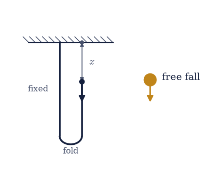
Fig. 102 A folded chain: the left strand is fixed to the ceiling, the right (free) end is released from the top and has fallen a distance \(x\) (marked), with links peeling through the fold at the bottom onto the fixed strand. A reference mass (right) is released simultaneously in free fall under \(g\); the chain’s free end outruns it.

Solution — Act III

v²/2gx rises from 1.000 (small x) to 5.405 (x≈0.9L)

Validation — Act III (parts 3, 4)

✓  the integrated EOM matches the energy-conserving v²(x)   [max|Δ| = 4.94417e-09 (rtol=1e-06, atol=1e-09)]
✓  the folded chain's free end falls faster than free fall   [v²/2gx in [1.00, 5.41]]

True

Part 5 — the energy gap. The energy-conserving chain keeps \(E=E_0\). The inelastic-fold model instead lets the moving strand free-fall (\(v^2=2gx\)) and dissipates the difference. Comparing the kinetic energies of the two models at the same configuration gives a clean closed form for the gap, \(\Delta E(x) = \tfrac14\lambda g x^2 > 0\): the energy the inelastic fold would destroy, and exactly what the energy-conserving fold instead supplies as work.

energy gap at x=0.9L: 1.9780 J;  ¼λgx² = 1.9780 J

✓  the folded-chain idealisations disagree — energy is lost at an inelastic fold   [gap(x≈0.9L) = 1.9780 J]
✓  the energy gap is exactly ¼λgx²   [max|Δ| = 6.66134e-16 (rtol=1e-06, atol=1e-09)]

True

Exercise 4 — Animate the folded chain beside a free-fall mass (worked)

Motion is the whole point here, so this one is genuinely an animation: watch the folded chain fall while a mass dropped at the same instant free-falls beside it, and see the chain’s free end pull ahead. The validation checks the physics of the animated data (the free end’s lead over the reference), not the drawing.

Once Loop Reflect

Fig. 103 Animation of a folded chain falling (dark: the fixed strand, the shrinking moving strand, and the fold) beside a mass released simultaneously in free fall (amber): the chain’s free end (marked) outruns the free-fall mass, because links peeling through the fold drive it faster than \(g\) (Eq. eq-folded).

Validation — Exercise 4

At every instant the chain’s free end has fallen farther than the free-fall mass.

✓  the chain end stays ahead of the free-fall reference   [min lead = 0.0000 m, max lead = 0.206 m]

True

Exercise 5 — The free-end acceleration (student exercise)

No animation here: the lesson is a curve, not a motion. The acceleration \(a(x)\) of Eq. 127 is the momentum route’s prediction for the free end, and it is unbounded: it exceeds \(g\) at every \(x>0\) and diverges as the chain straightens, \(x\to L\).

1. Evaluate \(a(x)\) on a grid \(x\in(0, 0.95L)\) (numpy.linspace) with the a_folded you wrote in Act III, and plot \(a/g\) versus \(x/L\).

2. Confirm with numpy.all that \(a > g\) throughout, and that \(a\to\infty\) as \(x\to L\). Relate the runaway to the energy the fold must supply ever faster as the moving strand shortens.

A ✗ points at the \(a(x)\) expression, not at any drawing.

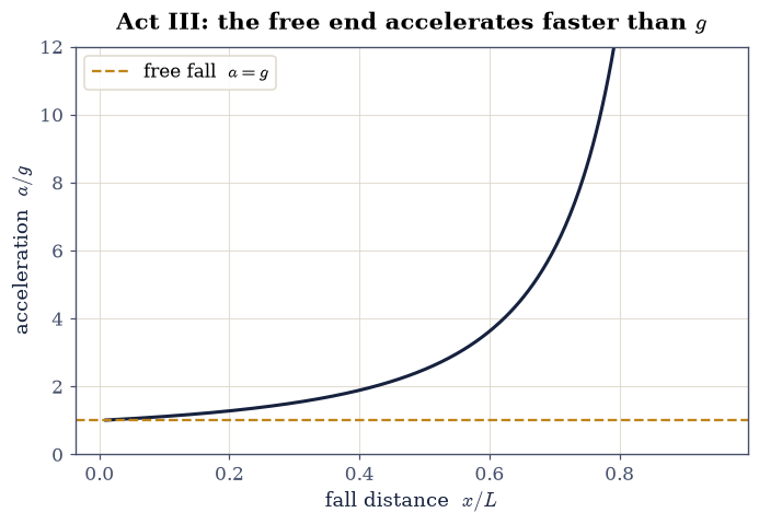
a/g ranges from 1.010 (small x) to 200.5 (x=0.95L)

✓  the free-end acceleration exceeds g everywhere   [min a/g = 1.010]

True

Exercise 6 — Act IV: the chain in reverse, or the rocket equation

Every act so far gathered mass; the rocket sheds it, and the same Eq. 123 bookkeeping — momentum carried across a moving boundary, never \(F = ma\) on a quietly changing mass — delivers the most consequential formula in astronautics. Ejecting propellant at exhaust speed \(v_e\) (relative to the rocket) at rate \(\mu = -dm/dt\) gives \(m\,\dot v = v_e \mu\), and integrating from mass \(m_0\) to \(m_1\),

(128)\[\Delta v \;=\; v_e \ln\frac{m_0}{m_1}\]

— Tsiolkovsky’s equation, with its tyrannical logarithm: a mass ratio of \(10\) buys only \(2.3\,v_e\).

1. Integrate \(\dot v = v_e\mu/m(t)\) with scipy.integrate.solve_ivp (\(v_e = 3\ \mathrm{km\,s^{-1}}\), \(m_0/m_1 = 10\), constant \(\mu\)) and verify Eq. 128 to rtol=1e-9.

2. Launch it vertically: add \(-g\) to the integrand and verify the closed form \(v = v_e\ln(m_0/m_1) - g\,t_{\rm burn}\) to the same tolerance. The gravity loss \(g\,t_{\rm burn} = 1766\ \mathrm{ m\,s^{-1}}\) eats a quarter of the free-space budget: every second spent burning is a second spent hovering, which is why real rockets throttle up and pitch over early.

3. The single-stage ceiling: give the rocket a structure fraction \(s = 0.10\) (tanks and engines are a tenth of each stage’s mass — they cannot be burned) and a payload of \(1\%\), and verify that even with zero payload \(\Delta v \le v_e \ln(1/s) = 6908\ \mathrm{m\,s^{-1}}\), while with the payload it reaches only \(6649\ \mathrm{m\,s^{-1}}\) (rtol=1e-2) — short of the \(\approx 9\ \mathrm{km\,s^{-1}}\) that reaching orbit costs.

4. Why rockets have stages: split the same total mass into two stages, optimize the split with scipy.optimize.minimize_scalar, and verify \(\Delta v = 9964\ \mathrm{m\,s^{-1}}\) (rtol=1e-2). Dropping the first stage’s dead structure mid-flight beats any single stage built from identical parts: orbit is unreachable in one piece and comfortable in two — the entire architecture of spaceflight, from one logarithm.

Tsiolkovsky: numeric vs closed, rel. gap 4.9e-12
with gravity: rel. gap 4.4e-12; gravity loss 1766 m/s of 6908
single stage: 6649 m/s (ceiling 6908); two stages (upper = 0.090): 9964 m/s

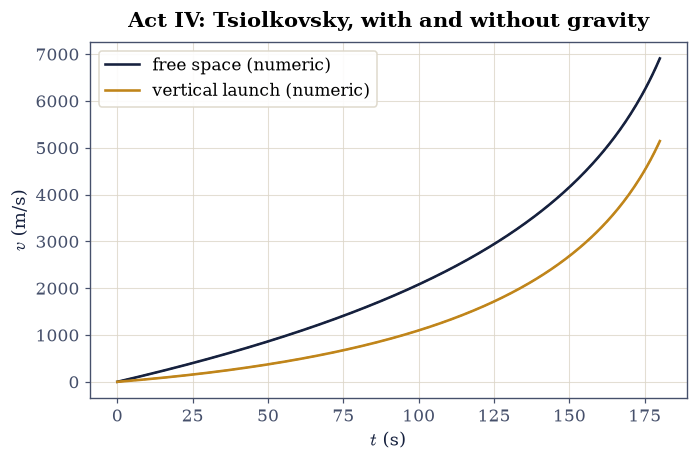
Fig. 104 Act IV, the chain’s bookkeeping pointed upward: velocity of a rocket with exhaust speed \(v_e = 3\ \mathrm{km\,s^{-1}}\) and mass ratio \(10\), integrated numerically (solid) against the closed forms (dashed) — Tsiolkovsky’s \(v_e\ln(m_0/m)\) in free space (ink) and the same minus \(gt\) for a vertical launch (amber), agreeing to \(10^{-9}\). The widening gap between the curves is the gravity loss, \(1766\ \mathrm{m\,s^{-1}}\) by burnout: a quarter of the budget, spent hovering.

✓  the integrated variable-mass dynamics lands on Tsiolkovsky's logarithm — and on its gravity-loss correction — to nine digits   [relative gaps 4.9e-12, 4.4e-12]
✓  the vertical burn spends a quarter of its budget hovering: gravity loss is why rockets pitch over early   [got [0.25562573] vs expected [0.2557] (rtol=0.01, atol=1e-09)]
✓  with 10% structure, orbit (~9 km/s) is unreachable in one piece even with zero payload — and comfortable in two: why rockets have stages   [single 6649 (ceiling 6908) vs staged 9964 m/s]
✓  with both architectures' budgets pinned to the metre per second   [max|Δ| = 0.387241 (rtol=0.01, atol=1e-09)]

True

Notebook summary

Three chains, three failures of “just gravity”:

• Act I: the sliding chain accelerates as \(\ddot x=(g/L)x\) and grows like a \(\cosh\); nothing is jerked, so energy and momentum agree.

• Act II: the piling chain makes the floor read three times the landed weight, because stopping the arriving links costs an extra \(2\lambda y g\); energy is plainly dissipated.

• Act III: the folded chain’s free end falls faster than \(g\); whether energy is conserved hinges on how the fold negotiates the links, and the two idealisations differ by exactly \(\tfrac14\lambda g x^2\).

And Act IV ran the bookkeeping in reverse — mass shed instead of gathered — and got Tsiolkovsky’s \(\Delta v = v_e\ln(m_0/m_1)\) to nine digits, the \(1766\ \mathrm{m\,s^{-1}}\) gravity loss of a vertical burn, and the staging argument: with \(10\%\) structure, orbit is unreachable in one piece (\(6649\) of \(9000\ \mathrm{m\,s^{-1}}\)) and comfortable in two (\(9964\)).

The single thread is Eq. 123: \(\mathbf F_\text{ext}=d\mathbf p/dt\) for the whole system, applied with the momentum carried across the moving boundary, not \(F=ma\) on a mass that is quietly changing.

Outlook

• The chain fountain (Mould effect): a chain that leaps above its beaker as it pours out: a modern variable-mass puzzle with a momentum-flux explanation.

• Beyond Exercise 6’s rocket: real ascent trajectories add drag, pitch programs, and the gravity turn — the \(d\mathbf p/dt\) bookkeeping is the same, wrapped in an optimal-control problem.

• The catenary, the static hanging chain, is a problem in the calculus of variations: the tool of §2.8.

References

[Nol16]

Wolfgang Nolting. Theoretical Physics 1: Classical Mechanics. Springer, 2016. Grundkurs Theoretische Physik 1.

Take this notebook with you

Use the download button (↓) in the toolbar above to save this notebook and run it yourself. The published notebooks ship without worked solutions; if you would like the reference solutions — to teach from or to check your own work — get in touch: hello@ramador.me.