


1.6 Symplectic vs. Naive Integrators#
Notebook overview#
Throughout Volume I we used energy conservation as a check on our integrators: the double pendulum (§1.3), the Kepler orbit (§1.4), and the coupled chain (§1.5) were all certified by watching their total energy hold steady to ten or eleven digits. We trusted those checks. This capstone turns the running theme into the subject itself and asks the question underneath it: why do some integrators deserve that trust over long times while others (even very accurate ones) do not?
The answer is geometric. A good long-time integrator is one that preserves the right structure of the flow, not merely the one with the smallest per-step error. We will see that the humble velocity-Verlet scheme, only second-order accurate, keeps the energy of a harmonic oscillator bounded for millions of steps, while the fourth-order Runge–Kutta (RK4) method (far more accurate per step) slowly bleeds energy away. The distinguishing property is symplecticity: preservation of phase-space area.
We will (1) implement four steppers, (2) run the headline energy comparison over many periods, (3) show Euler’s energy grows by exactly \((1+h^2)\) per step, (4) show Verlet’s energy error is bounded, not merely small, (5) measure each method’s order of accuracy, (6) animate a blob of initial conditions to see phase-space area preserved or destroyed, and (7) apply the methods to a Kepler orbit, where a symplectic step keeps the ellipse closed while Euler spirals out.
How to read the checks. Each exercise ends with a validation that compares our result to an expected physical fact. A ✗ does not by itself mean the answer is wrong: it means the output didn’t match what the check expected, which may be a real error, a different-but-valid convention (a sign, a unit, an array order), or simply too tight a tolerance. Treat a ✗ as a prompt to locate the discrepancy; passing is strong evidence of correctness, not proof.
Scope. This is a working review, not a textbook chapter. For the mechanics see Nolting, Theoretical Physics 1 [Nol16]; for the full geometric-integration picture (symplectic maps, modified shadow Hamiltonians, backward error analysis), see Hairer, Lubich & Wanner, Geometric Numerical Integration [HLW06].
Theory in brief#
The test system: the harmonic oscillator#
We test every method on the system whose exact answer we know completely: the unit harmonic oscillator \(\dot q = p\), \(\dot p = -q\) (mass \(m=1\), frequency \(\omega=1\)). Its energy is
the exact period is \(2\pi\), and the exact trajectory is a rotation of the phase-space point \((q,p)\) at unit angular rate: a circle of constant radius \(\sqrt{2E}\). Any drift in that radius is purely the integrator’s fault, which is what makes this system the perfect proving ground.
A one-step integrator advances \((q_n, p_n) \mapsto (q_{n+1}, p_{n+1})\) by a fixed step \(h\). For a linear system each step is a matrix; the determinant of that matrix is the factor by which it scales phase-space area, and over long times it governs the energy trend as well: secular growth if the determinant exceeds 1, no net growth if it is exactly 1.
Explicit (forward) Euler#
The most naive scheme evaluates the slope at the old point:
Its step matrix is \(\bigl(\begin{smallmatrix} 1 & h \\ -h & 1 \end{smallmatrix}\bigr)\), with determinant \(1 + h^2 > 1\). Every step inflates phase-space area (and energy) by the factor \(1+h^2\), so after \(n\) steps the energy is \((1+h^2)^n E_0\): an exponential blow-up, no matter how small \(h\) is. Forward Euler is first-order accurate (\(O(h)\) global error) and not symplectic.
Symplectic (semi-implicit) Euler#
A one-character change rescues it: update \(p\) first, then use the new \(p\) to update \(q\),
The step matrix is now \(\bigl(\begin{smallmatrix} 1-h^2 & h \\ -h & 1 \end{smallmatrix}\bigr)\), with determinant exactly 1. The method is area-preserving (symplectic), though still only first-order accurate. It does not conserve \(E\) exactly, but it conserves a nearby modified energy, so the true energy merely oscillates within a bounded band.
Velocity Verlet#
The workhorse of molecular dynamics splits each step into a half-kick, a full drift, and a half-kick:
Velocity Verlet is second-order accurate and symplectic (step determinant exactly 1). Crucially it conserves a shadow Hamiltonian that differs from the true \(E\) by \(O(h^2)\), so the true energy stays bounded and oscillatory with no secular drift: bounded forever, not just initially small.
Runge–Kutta 4#
The classic fourth-order scheme combines four slope evaluations:
with \(\mathbf k_1 = f(\,\cdot_n\,)\), \(\mathbf k_2 = f(\,\cdot_n + \tfrac{h}{2}\mathbf k_1)\), \(\mathbf k_3 = f(\,\cdot_n + \tfrac{h}{2}\mathbf k_2)\), \(\mathbf k_4 = f(\,\cdot_n + h\,\mathbf k_3)\) and \(f(q,p) = (p,-q)\). RK4 has a tiny per-step error (\(O(h^5)\)) but is not symplectic: its step determinant differs from 1 at \(O(h^6)\), so over very long runs the energy drifts secularly: slowly but without bound.
The lesson#
For long-time dynamics the geometry a method preserves can matter more than its order of accuracy. A symplectic method (Verlet, symplectic Euler) trades a little per-step accuracy for a structural guarantee (bounded energy) that a higher-order non-symplectic method (RK4) cannot offer. That is why the energy checks we trusted in §1.3–§1.5 were trustworthy there (an adaptive high-order solver over a modest number of periods) but would be the wrong tool for a billion-step molecular-dynamics run.
Setup#
Data and instruments only: the exact period of the unit oscillator, and a
run(stepper, h, n) driver that iterates whatever one-step map it is handed
and returns the trajectories Q, P and the energy series E. This
notebook’s own machinery is not here — the four steppers are its whole
subject, so you write step_euler, step_symplectic_euler, step_verlet and
step_rk4 in Exercise 1 and the rest of the notebook drives the ones you
wrote. Exercise 7 writes its own Euler and Verlet updates for the vector
\(1/r^2\) field of §1.4, which needs a two-component
state rather than the scalar (q, p) of the oscillator.
The Setup below holds this notebook’s data and instruments — nothing you are asked to build. It is collapsed so the building stays yours; expand it whenever you want the details.
Exercise 1 — Write the four steppers#
The four update rules of the theory section (forward Euler Eq. 119, symplectic Euler Eq. 120, velocity Verlet Eq. 121, and RK4 Eq. 122) are each a map \((q,p) \mapsto (q,p)\) on the unit oscillator \(\dot q = p\), \(\dot p = -q\), and every figure in the rest of this notebook is produced by one of them. The cleanest way to be sure they are transcribed correctly is to take a single step by hand from a known starting point and compare: from \((q,p)=(1,0)\) with \(h=0.1\), substituting into the formulas gives \((1,\,-0.1)\) for forward Euler; \((1-0.1\cdot0.1,\,-0.1) = (0.99,\,-0.1)\) for symplectic Euler; \((0.995,\,-0.0997\ldots)\) for velocity Verlet; and, for RK4, the exact rotation-by-\(h\) value \((\cos h,\,-\sin h)\) with its Taylor series truncated at fourth order, since the scheme reproduces the exact flow to \(O(h^5)\).
Part a) Write the four steppers step_euler(q, p, h),
step_symplectic_euler(q, p, h), step_verlet(q, p, h) and
step_rk4(q, p, h), each returning the updated (q, p). Give them the one
identical signature so any of them can be handed to the Setup’s run driver,
and write the bodies as plain arithmetic on q and p so that they also work
elementwise on NumPy arrays: Exercise 6 steps a whole ring of initial
conditions at once through the same functions. Write these yourself — the
implementations are the lesson of this notebook, and the difference between
Eq. 119 and Eq. 120 is one line of ordering.
Part b) Certify the transcription: take one step of size \(h=0.1\) from
\((q,p)=(1,0)\) with each method and check it against the hand computation
above, to rtol=1e-12.
forward Euler -> q=1.0000000000 p=-0.1000000000
symplectic Euler -> q=0.9900000000 p=-0.1000000000
velocity Verlet -> q=0.9950000000 p=-0.0997500000
RK4 -> q=0.9950041667 p=-0.0998333333
✓ one step of forward Euler matches the hand computation [max|Δ| = 0 (rtol=1e-12, atol=1e-09)]
✓ one step of symplectic Euler matches the hand computation [max|Δ| = 0 (rtol=1e-12, atol=1e-09)]
✓ one step of velocity Verlet matches the hand computation [max|Δ| = 0 (rtol=1e-12, atol=1e-09)]
✓ one step of RK4 matches the hand computation [max|Δ| = 1.38778e-17 (rtol=1e-12, atol=1e-09)]
Exercise 2 — Energy over many periods: the headline comparison#
This is the centrepiece: all four methods on the same oscillator, at the same fixed step \(h=0.05\), over about sixteen periods, with the energy Eq. 118 the only quantity watched. The theory makes sharp predictions: forward Euler Eq. 119 should blow up geometrically as \((1+h^2)^n\), RK4 Eq. 122 should sag almost imperceptibly, and the two symplectic methods should stay essentially flat.
Run each of the four steppers you wrote in Exercise 1 (forward Euler, symplectic Euler, velocity Verlet, RK4) at \(h=0.05\) for \(n\) steps covering \(\approx 16\) periods, and compute \(E(t)/E_0\) for each with the Setup’s
rundriver.Plot all four energy ratios on one axes (a log \(y\)-scale shows the four-decade spread). This single figure is the whole notebook in a picture.
Confirm Euler’s energy has blown up (final ratio \(> 10\)) while Verlet’s stays bounded (\(\max|E/E_0 - 1| < 10^{-3}\)).
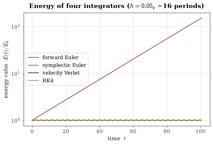
Euler final E/E0 = 151.60
Verlet max|E/E0-1| = 6.25e-04
✓ explicit Euler energy blows up over many periods [final E/E0 = 151.6]
True
✓ velocity-Verlet energy stays bounded [max|E/E0-1| = 6.25e-04]
True
Exercise 3 — Euler’s geometric energy growth#
The blow-up in Exercise 2 is not vague numerical noise; it is an exact, knowable rate. The step matrix of forward Euler Eq. 119 has determinant \(1+h^2\), and for this oscillator the energy Eq. 118 scales with phase-space area, so each step multiplies the energy by exactly \(1+h^2\). Iterating that one factor is precisely the \((1+h^2)^n\) exponential we just watched climb, so the entire blow-up is already contained in a single step, where it can be pinned down to machine precision instead of merely eyeballed on a log axis.
Take one step of size \(h=0.05\) from \((q,p)=(1,0)\) with the
step_euleryou wrote in Exercise 1, using the Setup’srundriver, whose energy series Eq. 118 holds \(E_0\) and \(E_1\) in its first two entries. Print the ratio \(E_1/E_0\) beside the predicted \(1+h^2\).Confirm the two agree to machine precision.
E[1]/E[0] = 1.002500000000
1 + h^2 = 1.002500000000
✓ Euler grows energy by exactly (1+h²) per step [got 1.0025 vs expected 1.0025 (rtol=1e-06, atol=1e-09)]
True
Exercise 4 — Verlet energy is bounded, not just small#
A method could have a small energy error that nonetheless creeps in one direction forever: that is secular drift, and it is what eventually ruins a long run. The symplectic guarantee is stronger than “small error”: it says the energy error of velocity Verlet Eq. 121 is bounded, oscillating within a fixed band that does not grow with time. RK4 Eq. 122, by contrast, has a far smaller error that nevertheless drifts.
Run the
step_verletyou wrote in Exercise 1 for a long run (\(\sim 20\,000\) steps) and compare the maximum relative energy deviation in the first half of the run to that in the second half (numpy.maxon each half). For a bounded (non-drifting) method they are equal.Run your Exercise 1
step_rk4over the same span and plot both energy series, so you can see Verlet’s steady ripple against RK4’s slow downward sag.
Verlet max|E/E0-1|, first half = 6.250000e-04
Verlet max|E/E0-1|, second half = 6.250000e-04
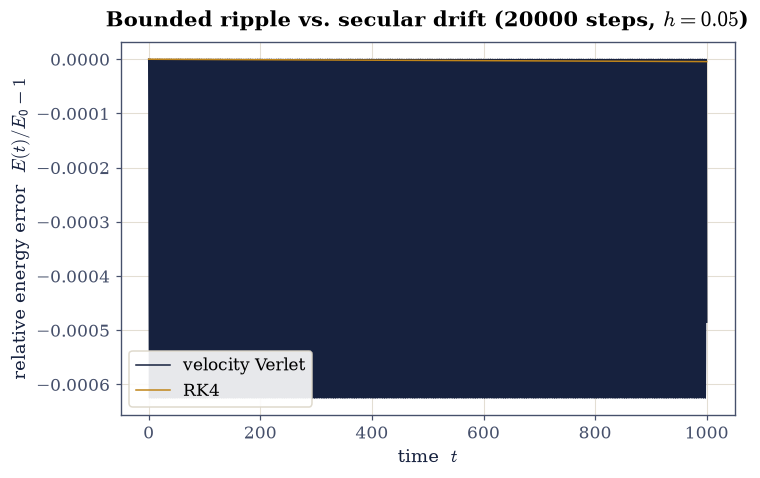
✓ Verlet energy error does not grow with time (bounded, not secular) [got 0.000625 vs expected 0.000625 (rtol=0.1, atol=1e-09)]
True
Exercise 5 — Order of accuracy#
Symplecticity governs long-time behaviour; the order of accuracy governs the per-step error and how fast it shrinks as \(h\to 0\). Euler Eq. 119 is first order, Verlet Eq. 121 second, RK4 Eq. 122 fourth. That number is readable as a slope. Started from \((q,p)=(1,0)\), the exact oscillator sits at \((\cos T, -\sin T)\) at time \(T\), so the global error \(\lvert(q,p)-(\cos T,-\sin T)\rvert\) measured at one fixed \(T\) across a range of step sizes falls like \(h^{\,\text{order}}\): a straight line on log–log axes whose slope is the order.
Measure at a generic time. Evaluate the error at \(T=10\), not at a multiple of the period \(2\pi\). At \(T=2\pi n\) the oscillator’s global error has a node where the leading error term vanishes, and the fitted order collapses to nonsense. This is a real subtlety, not a bug in the code: a ✗ here may just mean the measurement was at the wrong \(T\).
Integrate from \((q,p)=(1,0)\) to \(T=10\) with the
step_euler,step_verletandstep_rk4you wrote in Exercise 1, at the five step sizes \(h=0.1\), \(0.05\), \(0.025\), \(0.0125\), \(0.00625\) (\(n=T/h\) steps of the Setup’srundriver each time), and record every method’s global error against \((\cos T, -\sin T)\) at \(T\) (numpy.hypoton the two components of the difference).Plot the five errors against \(h\) for each method on log–log axes, and fit each method’s order as the slope of its line, with a degree-1
numpy.polyfiton \(\log h\) against \(\log(\text{error})\).Confirm the fitted orders come out near \(1\) for forward Euler, \(2\) for velocity Verlet and \(4\) for RK4.
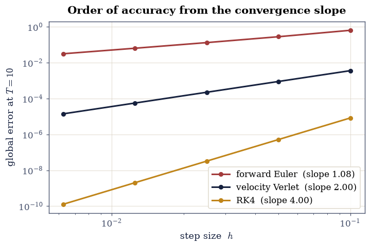
forward Euler fitted order = 1.083
velocity Verlet fitted order = 2.000
RK4 fitted order = 4.000
✓ forward Euler is first order [got 1.08318 vs expected 1 (rtol=1e-06, atol=0.15)]
True
✓ velocity Verlet is second order [got 2.00016 vs expected 2 (rtol=1e-06, atol=0.15)]
True
✓ RK4 is fourth order [got 3.99997 vs expected 4 (rtol=1e-06, atol=0.2)]
True
Exercise 6 — Phase-space area: the geometry behind it all (worked animation)#
Here is why symplectic methods conserve energy, made visible. Liouville’s
theorem says the exact flow of a Hamiltonian system preserves phase-space area:
a blob of initial conditions may distort in shape but never changes its area.
An integrator that respects this (a symplectic one) keeps energy bounded; one
that violates it does not. We take a small ring of initial conditions in
\((q,p)\) and evolve every point with the step_euler Eq. 119 and, separately,
the step_verlet Eq. 121 written in Exercise 1 — the same scalar
arithmetic, handed whole arrays of q and p instead of two floats.
The animation overlays the two evolving blobs. Euler’s inflates without bound (its area grows as \((1+h^2)^n\), exactly the energy factor of Exercise 3), while Verlet’s rotates rigidly with its area fixed. This is Liouville’s theorem violated vs. respected. This is the worked example for the two-animation rule; you build the second one in Exercise 7.
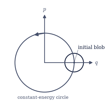
Fig. 96 Phase-space picture behind Liouville’s theorem: a blob of initial conditions (dark ring) in the position-momentum plane \((q,p)\) is carried by the exact Hamiltonian flow around the constant-energy circle (grey); the flow may distort the blob’s shape but, by Liouville’s theorem, never changes its enclosed area.#
Euler area: 0.2816 -> 0.9293 (×3.30; (1+h²)^n = 3.30)
Verlet area: 0.2816 -> 0.2816 (relative drift 2.5e-14)
Fig. 97 Animation of a ring of initial conditions in the \((q,p)\) plane of the harmonic oscillator evolved at step \(h=0.1\) by forward Euler (red) and velocity Verlet (blue): the Euler blob inflates without bound as its area grows like \((1+h^2)^n\), while the symplectic Verlet blob rotates rigidly at fixed area, Liouville’s theorem violated versus respected.#
✓ Verlet preserves phase-space area (symplectic) [max relative drift = 1.57712e-14 (limit 0.001)]
True
✓ Euler inflates phase-space area (violates Liouville) [area grew ×3.30]
True
Exercise 7 — Long-time orbit fidelity (student-implemented animation)#
The payoff for real physics: take the gravitational \(1/r^2\) force from §1.4 and integrate a bound elliptical orbit for many periods. The exact orbit is a closed ellipse: it should retrace itself forever. A symplectic step (velocity Verlet) keeps it closed; forward Euler, injecting energy every step, spirals the planet steadily outward. This is the same energy story as the oscillator, now with a recognisable orbit attached.
We reuse the inverse-square acceleration \(\ddot{\mathbf r} = -\mathbf r/r^3\) and the bound initial condition of §1.4 (\(\mathbf r_0=(1,0)\), \(\mathbf v_0=(0,1.2)\), in units \(GM=1\)). The energy is \(E=\tfrac12 v^2 - 1/r\).
Integrate the orbit for many periods with Euler and (separately) with velocity Verlet, both at the same small step (data prepared below). The Exercise 1 steppers act on a scalar pair \((q,p)\), so here the same two update rules Eq. 119, Eq. 121 are rewritten for a two-component \((\mathbf r, \mathbf v)\) state driven by the \(1/r^2\) acceleration rather than by \(-q\).
Build the animation comparing the two orbits side by side: you have the trajectories
(xe, ye)and(xv, yv); assemble aFuncAnimationthat traces both paths,plt.close(fig), then display withecp.animate.show. Target look: Verlet a clean closed ellipse, Euler a widening spiral.Quantify the story: confirm Verlet’s energy stays bounded over the run while Euler’s energy rises systematically (it injects energy).
A ✗ on the final checks is about the energy series we computed, not the animation: there are many valid ways to draw two orbits. If a check fails, inspect
E_verletandE_euler: the physics lives there, and any correctFuncAnimationdrawing the same data is fine.
Kepler orbit: a=1.7857, T=14.993, 20 periods, 29987 steps
Verlet energy relative drift = 2.82e-05
Euler energy change = +0.56 (of |E0|)