6.9 From Vectors to Wave Functions: The Position Representation and Continuous Spectra

Elementary Computational Physics

Volume VI — Quantum Mechanics Notebook 6.9

The same theory, infinitely many dimensions. A particle on a line has a state that is a function — the amplitude to be found at each point — and everything from the finite case carries over: sums become integrals, a Hermitian matrix becomes the operator −iℏ d/dx, and the change of basis to momentum is the Fourier transform. The price of the continuum is a new subtlety (eigenstates that cannot be normalized); the reward is that the uncertainty principle becomes Fourier reciprocity, and the Gaussian its sharpest state.

Level · advanced   •   Est. · 160–200 min

Raymond Amador v1.4.0  ·  2026-07-31  ·  CC BY 4.0 (text) / MIT (code)

Notebook overview

Every notebook so far has lived in a finite number of dimensions — two for a qubit, three or four for the small examples. This notebook opens Movement II by taking the same formalism to infinitely many dimensions, and the central message is one of reassurance: nothing here is a new postulate. Wave mechanics is not a rival theory to the vectors and operators we have been using; it is exactly that theory, written in a continuous basis. A particle on a line has a state \(|\psi\rangle\) whose “components” in the position basis form a wave function \(\psi(x)=\langle x|\psi\rangle\) — the amplitude to find the particle at \(x\) — and every structure of Movements 0–I carries straight over.

The translation is worth seeing as a table, because each line is a finite object we already know becoming its continuous cousin:

finite-dimensional (Movements 0–I)	infinite-dimensional (here)
components $c_i=\langle e_i	\psi\rangle$
inner product $\langle\phi	\psi\rangle=\sum_i\phi_i^{*}\psi_i$
normalization $\sum_i	c_i
resolution of the identity $\sum_i	e_i\rangle\langle e_i
a Hermitian matrix	a differential operator, \(\hat p=-i\hbar\,d/dx\)
change of basis (a unitary)	the Fourier transform

Two payoffs follow. The position and momentum operators obey the canonical commutator \([\hat x, \hat p]=i\hbar\) — the continuous cousin of the Pauli non-commutation of §6.6 — and feeding it into the Robertson relation of §6.6 derives the Heisenberg uncertainty principle \(\Delta x\,\Delta p\ge \hbar/2\), saturated by the Gaussian at every width (answering the forward pointer of §6.6). And the Fourier transform is revealed as nothing but the unitary change of basis between the position and momentum representations, so a state narrow in \(x\) is broad in \(p\): the uncertainty principle is Fourier reciprocity.

We are honest about the one genuinely new thing the continuum brings. The eigenstates of position and momentum — sharp points and plane waves — are not normalizable: they are idealized limits, not physical states, and this is exactly where the completeness we deferred in §6.1 finally bites. We name the rigorous home (the rigged Hilbert space) without belaboring it, and keep the physics in the normalizable wave packets.

As in every Volume VI notebook, each exercise opens with a crystal-clear statement and enumerated parts, each naming the exact operation — a discretized grid, numpy.fft.fft/ifft/fftfreq for the Fourier transform and the spectral-derivative momentum operator (with the normalization stated), and numpy.trapezoid for the expectation integrals.

Conventions. We set \(\hbar=1\). The grid is \(N\) points on \([-L/2,L/2)\) with spacing \(dx=L/N\); the conjugate (angular) wavenumber grid is \(k=2\pi\,\)numpy.fft.fftfreq(N, dx) and the momentum is \(p=\hbar k\). The momentum operator is the spectral derivative, \(\hat p\psi=\)ifft(ℏk· fft(ψ)). All numerical checks are made in the bulk, away from the periodic grid boundaries where the spectral derivative wraps around. The Schrödinger equation solved on this grid is §6.10; coherent states are §6.12; wave-packet dynamics is §6.13. See Sakurai & Napolitano (§1.6–1.7); Nolting; and Notebooks §6.1 (states, completeness), §6.2 (operators), §6.3 (change of basis), §6.5 (the Born rule), §6.6 (the uncertainty relation), and Volume II (canonical quantization).

Theory in brief

The wave function as continuous components

A particle on a line has a state whose components in the continuous position basis \(\{|x\rangle\}\) form the wave function,

(538)\[\psi(x)=\langle x|\psi\rangle,\qquad \langle\phi|\psi\rangle=\int\phi^{*}(x)\psi(x)\,dx,\qquad \int|\psi(x)|^2\,dx=1,\qquad \int|x\rangle\langle x|\,dx=I .\]

Born’s rule becomes a probability density: \(|\psi(x)|^2\,dx\) is the probability of finding the particle in \([x,x+dx]\) — the continuous version of the \(|c_i|^2\) of §6.1 and §6.5.

The position and momentum operators

In the position representation, position acts by multiplication and momentum by differentiation — the derivative being what the generator of translations must look like on wave functions, an identification Sakurai & Napolitano (§1.6) make precise:

(539)\[(\hat x\psi)(x)=x\,\psi(x),\qquad (\hat p\psi)(x)=-i\hbar\,\frac{d\psi}{dx} ,\]

both Hermitian (with decay at infinity). On a computer \(\hat x\) multiplies by the grid, and \(\hat p\) is the spectral derivative — multiply by \(\hbar k\) in Fourier space — the infinite-dimensional Hermitian operators of §6.2.

The canonical commutator

Apply \(\hat x\hat p-\hat p\hat x\) to any wave function and the product rule does the rest: \(-i\hbar\left[x\psi'-(x\psi)'\right]=i\hbar\,\psi\), one line of calculus from the operators above (§1.6 of Sakurai & Napolitano derives it basis-independently, from translations),

(540)\[[\hat x,\hat p]=i\hbar ,\]

the foundational relation of quantum mechanics: the continuous analogue of \([\sigma_x,\sigma_y]=2i \sigma_z\), and what canonical quantization promotes the classical Poisson bracket \(\{x,p\}=1\) into (Volume II; \(\hbar\to0\) recovers classical mechanics). Everything non-classical flows from it.

The position–momentum uncertainty relation

Feeding \([\hat x,\hat p]=i\hbar\) into the Robertson relation of §6.6 gives the Heisenberg uncertainty principle, now derived rather than postulated,

(541)\[\Delta x\,\Delta p\ \ge\ \frac{\hbar}{2},\qquad \text{saturated by the Gaussian } \psi(x)\propto e^{-x^2/4\sigma^2}\ \text{at every width} .\]

The Gaussian is the minimum-uncertainty state — the wave-mechanical cousin of the spin \(|{+}z\rangle\) of §6.6, and the seed of coherent states (§6.12).

The Fourier transform as the momentum representation

The momentum-space wave function is the Fourier transform of \(\psi(x)\),

(542)\[\varphi(p)=\langle p|\psi\rangle=\frac{1}{\sqrt{2\pi\hbar}}\int\psi(x)\,e^{-ipx/\hbar}\,dx ,\]

and the momentum basis \(\{|p\rangle\}\) is just another orthonormal basis. The Fourier transform is the unitary change of basis between position and momentum (§6.3); Parseval’s theorem is its norm-preservation. Conjugate widths (\(\Delta p\approx\hbar/2\Delta x\)) make the uncertainty principle literally Fourier reciprocity.

Continuous spectra and non-normalizable eigenstates

The genuinely new feature. The eigenstates of \(\hat x\) (points \(|x_0\rangle\)) and of \(\hat p\) (plane waves \(e^{ipx/\hbar}\), the de Broglie waves with \(\lambda=2\pi\hbar/p\)) are not square-integrable,

(543)\[\hat p\,e^{ip_0x/\hbar}=p_0\,e^{ip_0x/\hbar},\qquad \int|e^{ip_0x/\hbar}|^2dx=\infty,\qquad \langle x|x'\rangle=\delta(x-x'),\ \langle p|p'\rangle=\delta(p-p') .\]

They are idealized limits, \(\delta\)-normalized — and here the completeness deferred from §6.1 finally bites. The rigorous home is the rigged Hilbert space (named, not developed); physical states are normalizable wave packets.

Setup

Data and instruments only: the series palette, the conventions (\(\hbar=1\)) and the discretized grid every exercise works on, numpy.trapezoid under a short name, the normalization of §6.1 and the moment machinery of §6.5 — the expectation \(\langle\hat O\rangle\) and the spread \(\Delta O\) — restated here in their continuum form, and the Gaussian wave packet that every exercise takes as its specimen. The objects this notebook is named for are deliberately absent: you write the position and momentum operators in Exercise 2 and the transform to the momentum representation in Exercise 5.

The Setup below holds this notebook’s data and instruments — nothing you are asked to build. It is collapsed so the building stays yours; expand it whenever you want the details.

Show code cell source

Hide code cell source

import matplotlib.pyplot as plt
import numpy as np

from ecp import draw, validate

ACCENT, INK, SOFT = draw.ACCENT, draw.INK, draw.SOFT  # data: the series palette

HBAR = 1.0  # data: ℏ = 1 throughout

# data: a discretized grid on [−L/2, L/2): N points, spacing dx. The conjugate wavenumber grid is
# k = 2π·numpy.fft.fftfreq(N, dx); the momentum grid is p = ℏk. The momentum operator is the spectral
# derivative p̂ψ = ifft(ℏk·fft(ψ)) (the FFT normalization: numpy's fft/ifft are an inverse pair, so the
# round trip carries no extra factor). All checks are made in the BULK, away from the periodic edges.

N_GRID = 2048
L_BOX = 40.0
DX = L_BOX / N_GRID
X_GRID = -L_BOX / 2 + DX * np.arange(N_GRID)


# instrument: numpy.trapezoid under a short name — quadrature on a uniform grid was the lesson of
# §0.4, and here it is only the integral sign every norm, probability and expectation value below
# is written with.
def trapz(values, x):
    """Integrate ``values`` over the grid ``x`` with ``numpy.trapezoid`` (the trapezoidal rule)."""
    return np.trapezoid(values, x)


# built from scratch in §6.1 (Exercise 2, the unit vector |ψ⟩/‖ψ‖); restated here as an instrument
# in its continuum form, where the norm is √∫|ψ|²dx rather than numpy.linalg.norm.
def normalize(psi, x):
    """Return ``psi`` scaled so that $\\int|\\psi(x)|^2\\,dx=1$ {eq}`eq-wavefunction`.

    Divides by $\\sqrt{\\int|\\psi|^2dx}$ (the continuous version of dividing by the norm in §6.1); after
    this $|\\psi(x)|^2$ is a genuine probability density.
    """
    return psi / np.sqrt(trapz(np.abs(psi) ** 2, x))


# built from scratch in §6.5 (Exercise 3, the expectation value derived from the Born rule);
# restated here as an instrument in its continuum form. It takes the operator as an argument, so
# the x̂ and p̂ you build in Exercise 2 plug straight in.
def expectation(op, psi, x):
    """The expectation value $\\langle\\psi|\\hat O|\\psi\\rangle=\\int\\psi^{*}(\\hat O\\psi)\\,dx$ (§6.5).

    Applies the operator ``op(psi, x)`` and integrates against $\\psi^{*}$ with `numpy.trapezoid`; the
    result is real for a Hermitian operator.
    """
    return trapz(np.conj(psi) * op(psi, x), x).real


# built from scratch in §6.5 (Exercise 4, the variance and its vanishing on definite values);
# restated here as its square root, an instrument: Δx and Δp are the quantities this notebook
# bounds, not quantities it teaches you to form.
def uncertainty(op, psi, x):
    """The uncertainty $\\Delta O=\\sqrt{\\langle\\hat O^2\\rangle-\\langle\\hat O\\rangle^2}$ (§6.5, §6.6).

    Applies ``op`` twice for $\\langle\\hat O^2\\rangle$. For $\\hat x$ and the spectral $\\hat p$ this
    gives $\\Delta x$ and $\\Delta p$, whose product the uncertainty relation bounds.
    """
    mean = expectation(op, psi, x)
    mean_sq = trapz(np.conj(psi) * op(op(psi, x), x), x).real
    return np.sqrt(max(mean_sq - mean**2, 0.0))


# data: the specimen every exercise below is written in terms of — a literal transcription of the
# displayed Gaussian, with its centre x0, mean momentum p0 and width σ as given parameters.
def gaussian_packet(x, x0=0.0, p0=0.0, sigma=1.0):
    """A normalized Gaussian wave packet $\\propto e^{-(x-x_0)^2/4\\sigma^2}e^{ip_0x/\\hbar}$ {eq}`eq-xp-uncertainty`.

    Centered at $x_0$ with mean momentum $p_0$ and position width $\\sigma$ ($\\Delta x=\\sigma$). It is
    the minimum-uncertainty state, $\\Delta x\\,\\Delta p=\\hbar/2$.
    """
    psi = np.exp(-((x - x0) ** 2) / (4 * sigma**2)) * np.exp(1j * p0 * x / HBAR)
    return normalize(psi, x)

Exercise 1 — The wave function and its probability density

A particle on a line is described by a wave function \(\psi(x)\) sampled on a grid, and that function is nothing more exotic than a list of components: \(\psi(x)=\langle x|\psi\rangle\) are the amplitudes of \(|\psi\rangle\) in the continuous position basis, exactly as the \(c_i\) of §6.1 were its amplitudes in a finite one Eq. 538. Born’s rule reads the squared modulus as a probability density: once \(\int|\psi(x)|^2dx=1\), the quantity \(|\psi(x)|^2dx\) is the probability of finding the particle in \([x,x+dx]\), so the probability of finding it anywhere in a region is that density integrated over the region.

1. Set up the grid (X_GRID) and build a wave packet (a gaussian_packet).

2. Check the normalization \(\int|\psi|^2dx=1\) with numpy.trapezoid — the normalize helper restated from §6.1 is what put it there.

3. Read \(|\psi(x)|^2\) as the Born probability density — the continuous \(|c_i|^2\) of §6.1/§6.5.

4. Compute \(P(a<x<b)=\int_a^b|\psi|^2dx\) by integrating the density over the sub-grid with numpy.trapezoid.

∫|ψ(x)|² dx = 1.00000000   (normalized: probability density)
P(-2.0 < x < 1.0) = ∫ |ψ|² dx = 0.4816

Validation 1

✓  the wave function is normalized, ∫|ψ(x)|²dx=1; |ψ(x)|² is a probability density (the continuous Born rule)   [got 1 vs expected 1 (rtol=1e-06, atol=1e-09)]

True

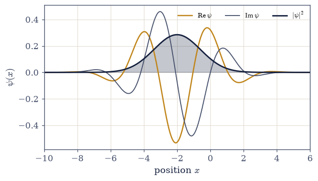
Fig. 528 A wave function on a line. A Gaussian wave packet carrying momentum: its real part (amber) and imaginary part (grey) oscillate at the de Broglie wavelength under a Gaussian envelope, while the probability density \(|\psi(x)|^2\) (ink, filled) is a smooth bump — the likelihood of finding the particle at each point. The wave function \(\psi(x)=\langle x|\psi\rangle\) is simply the list of the state’s components in the continuous position basis, exactly as a qubit’s two numbers were its components in \(\{|0\rangle,|1\rangle\}\); the only change is that the index \(x\) now runs over a continuum, so \(\sum_i\) has become \(\int dx\) and \(|c_i|^2\) has become the density \(|\psi(x)|^2\).

Exercise 2 — The position and momentum operators

In the position representation the two basic observables act in strikingly different ways: position acts by multiplication, \((\hat x\psi)(x)=x\,\psi(x)\), and momentum by differentiation, \((\hat p\psi)(x)=-i\hbar\,d\psi/dx\) Eq. 539. These are the infinite-dimensional Hermitian operators of §6.2, and Hermiticity (for wave functions that decay at infinity) obliges both to return real expectation values, so the vanishing of an imaginary part below is a check on the implementation and not a coincidence. On a grid the derivative is best taken spectrally: numpy.fft.fft and numpy.fft.ifft are an exact inverse pair carrying no extra factor, differentiation is multiplication by \(\hbar k\) in between, and the result is exact to machine precision in the bulk — wrapping around only at the periodic grid edges.

1. Write x_operator(psi, x), the position operator \(\hat x\psi=x\cdot\psi\) — multiplication by the grid, one line.

2. Write p_operator(psi, x), the momentum operator as the spectral derivative: build \(k=2\pi\,\) numpy.fft.fftfreq(N, dx) from the grid and return numpy.fft.ifft(ℏk * numpy.fft.fft(psi)). Write this one yourself — the implementation is the lesson.

3. Compute \(\langle x\rangle\) and \(\langle p\rangle\) with the expectation helper (\(\int\psi^{*}\hat O\psi\,dx\) via numpy.trapezoid).

4. Confirm both are real (the imaginary parts vanish — Hermitian operators) and match the packet’s centre \(x_0\) and mean momentum \(p_0\).

⟨x⟩ = -2.0000  (packet centre x0 = −2.0);  Im = -8.7e-19
⟨p⟩ = 1.5000  (mean momentum p0 = 1.5);   Im = 6.9e-18

Validation 2

✓  position multiplies and momentum differentiates (p̂=−iℏd/dx via the spectral derivative); both ⟨x⟩ and ⟨p⟩ are real

True

Exercise 3 — The canonical commutator \([\hat x,\hat p]=i\hbar\)

Multiplication and differentiation do not commute, and the product rule says exactly by how much: applying \(\hat x\hat p-\hat p\hat x\) to any wave function gives \(-i\hbar[x\psi'-(x\psi)']=i\hbar\psi\), so \([\hat x,\hat p]=i\hbar\) Eq. 540 — one line of calculus, and the foundational relation of quantum mechanics. Numerically the identity is exact only in the bulk of the grid: the spectral derivative wraps around at the periodic edges, so the middle half is where the two orderings can be fairly compared.

1. Take a smooth wave packet and compute \(\hat x\hat p\psi\) (apply the p_operator you built in Exercise 2, then multiply by \(x\)) and \(\hat p\hat x\psi\) (multiply by \(x\) first, then apply it).

2. Form the commutator \([\hat x,\hat p]\psi=\hat x\hat p\psi-\hat p\hat x\psi\).

3. Confirm it equals \(i\hbar\psi\) in the bulk by checking the ratio \([\hat x,\hat p]\psi/(i\hbar\psi)\approx1\).

4. Note this is the continuous analogue of the Pauli non-commutation of §6.6 and the quantization of \(\{x,p\}=1\) (Volume II). Everything non-classical flows from it.

[x̂,p̂]ψ / (iℏψ) in the bulk:  mean = 1.000000,  std = 4.7e-07
→ [x̂,p̂] = iℏ  (the continuous cousin of [σx,σy]=2iσz, and the quantization of {x,p}=1)

Validation 3

✓  the canonical commutator [x̂,p̂]=iℏ holds (verified in the bulk of the grid)   [got 1 vs expected 1 (rtol=0.001, atol=1e-09)]

True

Exercise 4 — The position–momentum uncertainty relation

The Heisenberg uncertainty principle is not a separate postulate in this course; it is what the Robertson relation of §6.6 returns when the commutator fed into it is the canonical one. With \(\Delta A\,\Delta B\ge\tfrac12|\langle[A,B]\rangle|\) and \([\hat x,\hat p]=i\hbar\), the right-hand side is the constant \(\hbar/2\), so \(\Delta x\,\Delta p\ge\hbar/2\) for every state whatsoever Eq. 541. Gaussians sit exactly on that floor; a state built from two separated bumps is a good way to see that generic states sit well above it.

1. Compute \(\Delta x=\sqrt{\langle\hat x^2\rangle-\langle\hat x\rangle^2}\) with the uncertainty helper applied to the x_operator you built in Exercise 2.

2. Compute \(\Delta p\) likewise with your Exercise 2 p_operator (the spectral derivative).

3. Form the product \(\Delta x\cdot\Delta p\) for several Gaussian widths and confirm it is \(\ge\hbar/2\).

4. Do the same for a two-bump superposition and see it land strictly above the bound — Heisenberg’s principle is a theorem about the commutator, and only special states make it an equality.

narrow  (σ=0.8): Δx = 0.8000, Δp = 0.6250, Δx·Δp = 0.5000  (≥ ℏ/2 = 0.5)
medium  (σ=1.4): Δx = 1.4000, Δp = 0.3571, Δx·Δp = 0.5000  (≥ ℏ/2 = 0.5)
broad   (σ=2.5): Δx = 2.5000, Δp = 0.2000, Δx·Δp = 0.5000  (≥ ℏ/2 = 0.5)
two-bump packet: Δx·Δp = 0.7692  (well above ℏ/2 — not a minimum-uncertainty state)

Validation 4

✓  the position–momentum uncertainty relation Δx·Δp ≥ ℏ/2 follows from [x̂,p̂]=iℏ (Robertson, §6.6)

True

Exercise 5 — The Gaussian: the minimum-uncertainty state

The inequality of Exercise 4 becomes an equality for the Gaussian, and it does so at every width: \(\Delta x=\sigma\) and \(\Delta p=\hbar/2\sigma\), so squeezing the packet in position widens it in momentum by exactly the reciprocal factor and the product stays pinned at \(\hbar/2\) Eq. 541. That makes the Gaussian the wave-mechanical analogue of the spin \(|{+}z\rangle\) of §6.6 and the seed of the coherent states of §6.12.

Watching that trade-off means seeing both sides of it at once, and the bridge between them is the Fourier transform: the momentum-space wave function is \(\varphi(p)=(2\pi\hbar)^{-1/2}\int\psi(x) e^{-ipx/\hbar}dx\) Eq. 542. Turning that integral into an FFT on this grid takes two pieces of bookkeeping — the factor \(dx/\sqrt{2\pi\hbar}\) that makes the transform unitary, and the phase \(e^{-ipx_0/\hbar}\) that accounts for the grid beginning at \(x_0=-L/2\) rather than at the origin — and one tidying step, since numpy.fft.fftfreq returns its wavenumbers in the wrapped FFT order and a plot wants them ascending.

1. Write to_momentum(psi, x), returning \(\varphi(p)\) and the ascending grid \(p=\hbar k\): take numpy.fft.fft(psi), apply the unitary factor and the offset phase above, and sort by \(p\). Write this one yourself — the implementation is the lesson.

2. Build Gaussians \(\psi\propto e^{-x^2/4\sigma^2}\) of several widths \(\sigma\) with gaussian_packet.

3. For each, compute \(\Delta x\) and \(\Delta p\) with the uncertainty helper and your Exercise 2 operators.

4. Confirm \(\Delta x=\sigma\), \(\Delta p=\hbar/2\sigma\), and the product \(\Delta x\cdot\Delta p=\hbar/2\) exactly.

5. Draw the trade-off with your to_momentum: the position densities beside the momentum densities, narrow in \(x\) against broad in \(p\), the product never beating \(\hbar/2\).

σ = 0.6:  Δx = 0.6000 (=σ),  Δp = 0.8333 (=ℏ/2σ),  Δx·Δp = 0.5000
σ = 1.0:  Δx = 1.0000 (=σ),  Δp = 0.5000 (=ℏ/2σ),  Δx·Δp = 0.5000
σ = 1.6:  Δx = 1.6000 (=σ),  Δp = 0.3125 (=ℏ/2σ),  Δx·Δp = 0.5000
σ = 2.5:  Δx = 2.5000 (=σ),  Δp = 0.2000 (=ℏ/2σ),  Δx·Δp = 0.5000
σ = 4.0:  Δx = 4.0000 (=σ),  Δp = 0.1250 (=ℏ/2σ),  Δx·Δp = 0.5000
every width saturates Δx·Δp = ℏ/2 = 0.5

Validation 5

✓  the Gaussian is the minimum-uncertainty state: Δx·Δp = ℏ/2 at every width   [max|Δ| = 3.22729e-06 (rtol=1e-06, atol=0.02)]

True

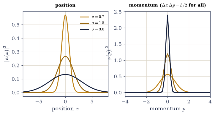
Fig. 529 The Gaussian saturates the bound at every width. Left: three Gaussian wave packets, narrow to broad, with their position spreads \(\Delta x=\sigma\). Right: the corresponding momentum distributions \(|\varphi(p)|^2\) — a narrow packet in \(x\) is a broad one in \(p\) and vice versa, the spreads trading off as \(\Delta p=\hbar/2\sigma\). Yet the product \(\Delta x\,\Delta p\) is pinned at exactly \(\hbar/2\) for all of them (inset values): the Gaussian is the wave-mechanical minimum-uncertainty state, the continuous cousin of the spin \(|{+}z\rangle\) that saturated the relation in §6.6. The reciprocity of the two widths is the uncertainty principle, and it is nothing but a property of the Fourier transform.

Exercise 6 — The Fourier transform as the momentum representation

The momentum basis \(\{|p\rangle\}\) is just another orthonormal basis, and the transform you built in Exercise 5 is the unitary change of basis between it and the position basis — the continuous cousin of the basis changes of §6.3 Eq. 542. A unitary leaves two things invariant, and both are checkable here: the norm, which is Parseval’s theorem \(\int|\varphi(p)|^2dp= \int|\psi(x)|^2dx=1\), and the expectation value of an observable, so \(\langle p\rangle\) must come out the same whether it is computed as \(\int\psi^{*}\hat p\psi\,dx\) in position space or as \(\int p\,|\varphi(p)|^2dp\) in momentum space. Once that is established, the conjugate widths of the two pictures make the uncertainty principle literally Fourier reciprocity.

1. Compute \(\varphi(p)\) with the to_momentum you wrote in Exercise 5, on the momentum grid \(p=\hbar k\).

2. Verify Parseval: \(\int|\varphi(p)|^2dp=\int|\psi(x)|^2dx=1\) (numpy.trapezoid).

3. Verify \(\langle p\rangle\) agrees across the two representations — the expectation of your Exercise 2 p_operator against \(\int p\,|\varphi(p)|^2dp\).

4. Show conjugate widths: a narrow packet in \(x\) is broad in \(p\).

Parseval: ∫|φ(p)|² dp = 1.000000  (= ∫|ψ(x)|² dx = 1, unitary)
⟨p⟩ from x-rep (−iℏd/dx) = 2.0000;   ⟨p⟩ from p-rep (∫p|φ|²dp) = 2.0000
  σ=0.7: Δx = 0.700, Δp = 0.714  (narrow x ↔ broad p)
  σ=2.0: Δx = 2.000, Δp = 0.250  (narrow x ↔ broad p)

Validation 6

✓  the Fourier transform is the unitary position↔momentum change of basis: Parseval (norm preserved) and ⟨p⟩ agree across representations   [max|Δ| = 4.44089e-16 (rtol=0.01, atol=1e-09)]

True

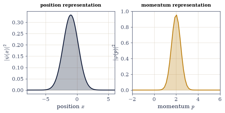
Fig. 530 One state, two representations. The same wave packet shown in the position representation \(|\psi(x)|^2\) (left, ink) and the momentum representation \(|\varphi(p)|^2\) (right, amber), connected by the Fourier transform — the unitary change of basis between \(\{|x\rangle\}\) and \(\{|p\rangle\}\), exactly as a qubit could be written in the \(z\)- or \(x\)-basis (§6.3). The packet sits near \(x=-1\) with mean momentum \(p\approx2\), and the two pictures carry identical physics: the norm is one in both (Parseval), and \(\langle p\rangle\) is the same computed either way. Schrödinger’s wave mechanics and Heisenberg’s matrices, which felt like rival theories in 1926, are just these two bases — and this transform is the unitary that relates them.

Exercise 7 — Momentum eigenstates, de Broglie, and the continuous spectrum (student)

The plane wave \(\psi(x)=e^{ip_0x/\hbar}\) is the eigenstate of \(\hat p\) with eigenvalue \(p_0\), and its spatial period is de Broglie’s wavelength \(\lambda=2\pi\hbar/p_0\) Eq. 543. It is also the genuinely new feature of the continuum, and an honest embarrassment: its modulus is \(1\) everywhere, so \(\int|\psi|^2dx\) is proportional to the size of the box and diverges as the box grows. A continuous-spectrum eigenstate is therefore not a physical state at all but a \(\delta\)-normalized idealization, whose rigorous home is the rigged Hilbert space (named here, not developed) — and this is exactly where the completeness deferred in §6.1 finally bites. Physical states remain the normalizable wave packets, which are superpositions of these idealizations.

1. Build the plane wave \(\psi(x)=e^{ip_0x/\hbar}\) on the grid.

2. Apply the p_operator you built in Exercise 2 and confirm in the bulk that \(\hat p\psi=p_0\psi\).

3. Compute the de Broglie wavelength \(\lambda=2\pi\hbar/p_0\).

4. Integrate \(|\psi|^2\) over boxes of growing length and watch the result grow with \(L\) — the plane wave is non-normalizable, and no rescaling repairs it.

p̂ψ / ψ in the bulk = 1.9999   (eigenvalue p0 = 2.0)
de Broglie wavelength λ = 2πℏ/p = 3.1416
  box L=  20: ∫|ψ|² dx = 20.0   (∝ L → diverges: not normalizable)
  box L=  40: ∫|ψ|² dx = 40.0   (∝ L → diverges: not normalizable)
  box L=  80: ∫|ψ|² dx = 80.0   (∝ L → diverges: not normalizable)
→ a momentum eigenstate is a continuous-spectrum, δ-normalized idealization; physical states are wave packets.

Validation 7

✓  a plane wave e^{ip₀x/ℏ} is a momentum eigenstate (de Broglie); it is non-normalizable — the continuous spectrum, δ-normalized (the rigged Hilbert space)   [got 1.99992 vs expected 2 (rtol=0.01, atol=1e-09)]

True

Exercise 8 — Wave mechanics is the same mechanics (synthesis)

Nothing in this notebook was a new postulate. The wave function is the state vector’s components in the position basis, \(\psi(x)=\langle x|\psi\rangle\); the inner product is an integral; the momentum operator is a derivative, \(\hat p=-i\hbar\,d/dx\); and the change to momentum is a Fourier transform. Every line of the bridge table from the overview is a finite object we already had, grown to a continuum. The one genuinely new thing — the continuous spectrum — cost us normalizability for the idealized position and momentum eigenstates and gave us, in return, the uncertainty principle as Fourier reciprocity and the Gaussian as its sharpest state.

There is no new computation to do here; the correspondence is the result. Schrödinger’s wave mechanics and Heisenberg’s matrices felt like rival theories for a year in 1926; they are the same theory in two bases, and the Fourier transform is the unitary that connects them — a fact we just verified on a grid. With the position representation in hand, the next notebook (§6.10) writes the Schrödinger equation as a differential equation, discretizes it into a matrix, and solves it the way we solved every operator problem in Movement 0 — by diagonalizing. The arena has changed from two amplitudes to a continuum of them; the method has not changed at all.

Notebook summary

Wave mechanics as the same formalism in infinitely many dimensions — the opening of Movement II.

• The wave function Eq. 538: \(\psi(x)=\langle x|\psi\rangle\), the components in the position basis; \(\int|\psi|^2dx=1\) with \(|\psi(x)|^2\) a Born density; sums become integrals and the resolution of the identity becomes \(\int|x\rangle\langle x|dx=I\).

• The operators Eq. 539: \(\hat x\) multiplies by the grid, \(\hat p=-i\hbar\,d/dx\) is the spectral derivative (numpy.fft) — the infinite-dimensional Hermitian operators of §6.2.

• The canonical commutator Eq. 540: \([\hat x,\hat p]=i\hbar\) (verified in the bulk) — the continuous cousin of the Pauli non-commutation, the quantization of \(\{x,p\}=1\).

• Uncertainty Eq. 541: \(\Delta x\,\Delta p\ge\hbar/2\) derived from the commutator via Robertson (§6.6), saturated by the Gaussian at every width.

• The Fourier transform Eq. 542: the unitary position↔momentum change of basis (Parseval; \(\langle p\rangle\) agrees both ways) — the uncertainty principle as Fourier reciprocity.

• The continuous spectrum Eq. 543: plane waves are non-normalizable, \(\delta\)-normalized eigenstates (the rigged Hilbert space); physical states are wave packets — where the completeness deferral of §6.1 finally bites.

Wave mechanics is the same mechanics. The next notebook diagonalizes the Schrödinger operator on a grid; the method is the one from Movement 0, only the arena is new.

Outlook

• The Schrödinger equation on a grid (§6.10): the differential equation discretized to a matrix eigenproblem and solved by diagonalization — bound states and spectra.

• One-dimensional systems (§6.11), the harmonic oscillator and coherent states (§6.12), wave-packet dynamics (§6.13): split-step Fourier and Crank–Nicolson propagation.

• The rigged Hilbert space and the spectral theorem for continuous spectra (a horizon, named).

• Cross-reference §6.1 (states / completeness), §6.2 (operators), §6.3 (change of basis), §6.5 (the Born rule), §6.6 (uncertainty), Volume II (canonical quantization), and forward to §6.10–§6.13.

Take this notebook with you

Use the download button (↓) in the toolbar above to save this notebook and run it yourself. The published notebooks ship without worked solutions; if you would like the reference solutions — to teach from or to check your own work — get in touch: hello@ramador.me.