


5.17 Molecular Dynamics: Periodic Boundaries, Cutoffs, and Pressure#
Notebook overview#
The reader of this volume has, by now, written every part of a molecular-dynamics program without ever running one. Velocity Verlet was built from scratch in §1.6, with its symplecticity, its shadow Hamiltonian, and its measured order of accuracy. The \(O(N^2)\) pairwise force sum, written as one broadcast expression with no Python loop over pairs, is §1.8, along with the discipline of a reduced unit system. Maxwell-Boltzmann velocities, autocorrelation functions and the Green-Kubo integral are §5.11; collisions, mean free paths and an event-driven hard-disk gas are §5.12, whose closing page hands the subject forward in as many words. The parts are all here. Nobody has ever switched them on together.
That is not an accident of this course. It is the shape of the literature: the integrator is taught in the chapter on differential equations, the sampling in the chapter on Monte Carlo, and the two are rarely introduced to each other. Allen and Tildesley [AT17] divide the subject the same way, and the division is instructive: their molecular-dynamics chapter is integrators and ensembles, while periodic boundaries and neighbour lists wait for a later chapter, and structure and error analysis for a later one still. So this notebook is the assembly, and what it adds is precisely the layer that sits outside the integrator.
Five things are genuinely new here. We differentiate the Lennard-Jones potential and turn it into a force, which no notebook in this course has done (§0.13 used the 12-6 form only as a scalar function to hand a minimizer). We build a box with no walls at all and the minimum-image convention that makes it work, and we watch what happens to a simulation that forgets it. We truncate the potential at a finite range and discover that a cutoff must be shifted or the energy will not stand still. We measure the pressure from the trajectory through the virial, which this volume has never done even while deriving a full equation of state in §5.15. And we start a gas from a velocity distribution that is not Maxwell-Boltzmann and watch smooth Newtonian flow make it Maxwell-Boltzmann, with a statistical test rather than a glance. Along the way we build the error analysis that a correlated trajectory demands, because a mean without an honest bar on it is not a measurement.
Two scope decisions, both deliberate. We work in two dimensions, which is a choice with precedent rather than a shortcut: Gould, Tobochnik and Christian [GTC07] and Schroeder [Sch00] both teach molecular dynamics in 2-D for the stated reasons that it visualises directly, costs far less, and demonstrates every principle the three-dimensional case does. It also continues §1.8, whose solar system is coplanar. And we run NVE only, with no thermostat, which lets us say plainly a thing the introductory literature almost never says: velocity rescaling does not sample the canonical ensemble, and neither does the Berendsen scheme that generalizes it. Exercise 6 measures exactly how it fails. Frenkel and Smit [FS02] is the standard reference for everything deeper.
A note on reading the checks in this notebook: a validation compares a result to an expected physical fact. A ✗ does not by itself mean the answer is wrong; it means the output did not match what the check expected, which may be a genuine error, a different-but-valid convention, or too tight a tolerance. Treat a ✗ as a prompt to locate the discrepancy. Passing is strong evidence, not proof.
Theory in brief#
The pair potential, and the force it implies#
A neutral atom feels two things from a neighbour: a weak long-range attraction from correlated fluctuations of the two electron clouds, which decays as \(r^{-6}\), and a violent short-range repulsion once the clouds overlap and the Pauli principle objects. Lennard-Jones combined them in the form that has carried simulation since Rahman put it on a computer in 1964 [Rah64], choosing the repulsive exponent as the square of the attractive one because it is cheap to evaluate rather than because it is right:
Here \(\sigma\) is the distance at which \(u\) crosses zero and \(\varepsilon\) the depth of the well, whose minimum sits at \(r_{\min} = 2^{1/6}\sigma\). Everything in this notebook runs in reduced Lennard-Jones units, \(\varepsilon = \sigma = m = k_B = 1\), the same move as the astronomical units of §1.8: lengths in \(\sigma\), energies in \(\varepsilon\), temperature as \(T^\ast = k_BT/\varepsilon\), and time in \(\sigma\sqrt{m/\varepsilon}\). Argon fixes the scale at \(\varepsilon/k_B = 119.8\ \mathrm{K}\) and \(\sigma = 3.405\ \text{Å}\) if a physical number is wanted.
A potential is not yet a simulation. What the integrator needs is the force, and for a central pair potential that is \(-\,\mathrm{d}u/\mathrm{d}r\) along the line of centres. Differentiating Eq. 466 and writing the result in the vector form the code actually wants, with \(\mathbf r_{ij} = \mathbf r_i - \mathbf r_j\) and \(r = |\mathbf r_{ij}|\),
The bracket over \(r^2\) is written that way on purpose: every term needs only \(r^2\), so no square root is ever taken in the inner loop. The force vanishes at \(r_{\min}\), is repulsive (parallel to \(\mathbf r_{ij}\)) inside it, and attractive outside.
A box with no walls#
A few hundred atoms in a box are almost all surface. In a \(10 \times 10\) square arrangement, sixty-four of the hundred atoms touch an edge, so a simulation with walls measures the walls. The standard repair, older than most of the field, is to abolish the walls: the cell of side \(L\) is made periodic, tiled infinitely in every direction, so an atom that leaves the right edge re-enters at the left and no atom is ever at a boundary. The bulk is then modelled by a system with no surface at all.
Periodicity alone is not enough, and here is the part every introduction skips over in a sentence. Two atoms near opposite edges of the cell are, as coordinates, nearly \(L\) apart; as physics they are neighbours, because each sits beside a periodic image of the other. Under the minimum-image convention the interaction of \(i\) with \(j\) is taken with the single nearest of the infinitely many images of \(j\), which for a cubic or square cell is one line of arithmetic on each Cartesian component of the separation:
which returns the representative of \(d_\alpha\) in \([-L/2, L/2)\). The convention is consistent only if no atom interacts with two images of the same partner, which is why every cutoff must satisfy \(r_c \le L/2\): a constraint that ties the range of the potential to the size of the box, and quietly sets the cost of every simulation ever run.
The cutoff, and why it must be shifted#
Evaluating Eq. 466 for every pair is \(O(N^2)\) work, and beyond a few \(\sigma\) the potential is negligible: \(u(2.5\sigma)\) is \(-0.0163\,\varepsilon\), under two percent of the well depth. So the interaction is truncated at \(r_c = 2.5\sigma\), the value the field has used since Verlet [Ver67]. Truncation alone leaves a discontinuity of size \(u(r_c)\) at the cutoff, and a discontinuous potential is not the potential of any force: every pair that crosses \(r_c\) takes a step in the total energy, so the quantity we monitor to certify the integrator random-walks away for reasons that have nothing to do with the integrator. Shifting removes it:
which is continuous at \(r_c\), leaves the force unchanged everywhere (so the trajectory is identical), and makes \(K + U\) a genuine constant of the motion again. This truncated-and-shifted potential is a slightly different physical model from the full Lennard-Jones one, and honest practice says so: every number below refers to \(u_{\rm ts}\) with \(r_c = 2.5\), including the theoretical predictions it is checked against.
Temperature, with the correction nobody mentions#
Equipartition assigns \(\tfrac12 k_BT\) to each quadratic degree of freedom, so a two-dimensional gas of \(N\) atoms would seem to give \(\langle K\rangle = N k_B T\). It does not, because the total momentum is a constant of the motion that we set to zero when the run starts and that Newton’s third law then holds there forever. Two of the \(2N\) velocity components are therefore not free, and the honest thermometer is
The correction is \(1/N\), invisible at \(N = 10^{23}\) and worth \(1.6\%\) at the \(N = 64\) of this notebook. Two cautions come with Eq. 470. It is a time average, meaningful only once the system has equilibrated; the instantaneous \(2K/(2N-2)\) fluctuates by tens of percent and is not a temperature. And it is a microcanonical temperature, the one belonging to a system of fixed energy, which is why nothing in this notebook is at a fixed temperature at all.
Pressure from the virial#
There are no walls left to push on, so pressure cannot be measured as a wall force. It is measured instead from the virial, the configuration sum that Clausius introduced for exactly this purpose. For a pairwise potential in \(d\) dimensions the result, derived in Allen and Tildesley [AT17] and in Frenkel and Smit [FS02], is that the ideal-gas kinetic pressure is corrected by the pair forces:
In two dimensions \(V\) is an area and \(d = 2\). Repulsive pairs (\(\mathbf f_{ij}\) along \(+\mathbf r_{ij}\)) push \(W\) up and the pressure with it; attractive pairs pull it down. That single sentence is the whole content of the van der Waals equation of state of §5.15, which this volume derived analytically and never once measured. Here we measure it. The low-density behaviour is fixed by the second virial coefficient, which in two dimensions is the plane integral
computable to machine precision by quadrature and therefore an independent judge of the simulation.
The integrator, and what it is doing here#
The stepper is velocity Verlet, kick-drift-kick, built from scratch with its shadow Hamiltonian and its measured second-order convergence in §1.6:
We do not rebuild it. Reusing it is the point: the reader wrote it once, established there why it is the right tool for a long Hamiltonian run, and it now arrives as an instrument, one force evaluation per step, so that the new work can be the layer around it.
Error bars on a trajectory#
One last piece of theory, and the one the textbooks leave out. Since §5.8 the reader has known to discard the transient at the start of a chain before averaging anything, and that habit carries over here unchanged. What has never been priced is the correlation that survives the cut. A molecular-dynamics run hands back a correlated time series: the temperature two steps from now is very nearly the temperature now. Successive samples are not independent, so the familiar \(\sigma/\sqrt{n}\) is not the error on the mean. The correct statement is written with the integrated autocorrelation time \(\tau_{\rm int}\) of the normalized autocovariance \(\rho(t)\),
so a run of \(n\) samples is worth \(n_{\rm eff}\) independent ones and the naive bar is too small by \(\sqrt{2\tau_{\rm int}}\). The window \(W\) cannot be taken to infinity (the tail is pure noise) and is fixed by Sokal’s self-consistent rule, the smallest \(W\) with \(W \ge c\,\tau_{\rm int}(W)\) at \(c = 8\). Exercise 8 builds this and the blocking analysis that confirms it. Ambegaokar and Troyer [AT10] is the reference to read.
Setup#
Reduced Lennard-Jones units throughout, \(\varepsilon = \sigma = m = k_B = 1\), so masses never appear and an acceleration is a force. The data are the state point this notebook works at (the cutoff \(r_c = 2.5\), the step \(\Delta t = 0.004\), the target temperature \(T = 1.0\), the reference density \(\rho = 0.4\)), the series palette, and the deliberately non-Maxwellian initial velocities of Exercise 7, which are the specimen the problem hands us rather than anything to be built. The instruments are a lattice builder and the velocity-Verlet driver of §1.6, restated here so the notebook stands alone: the driver only iterates whatever force routine it is handed and records what that routine returns.
This notebook’s own machinery is not here. The Lennard-Jones pair force is Exercise 1, the minimum-image displacement Exercise 2, the force-energy-virial machine Exercise 3, the thermometer Exercise 4, and the correlation-time and blocking estimators Exercise 8. Every run below is driven by the routines built in those exercises.
The Setup below holds this notebook’s data and instruments — nothing you are asked to build. It is collapsed so the building stays yours; expand it whenever you want the details.
Exercise 1 — The Lennard-Jones pair force#
The 12-6 potential Eq. 466 has appeared in this course once before, in §0.13, purely as a scalar function with a minimum for a minimizer to find. Nothing has ever differentiated it. That step, from a potential to the vector force Eq. 467 that an integrator can use, is the first thing a molecular-dynamics program does and the first thing to get wrong, so it gets its own exercise and its own certification.
Two features of the implementation are worth stating before writing it. The inner loop of every molecular-dynamics code sees the squared separation \(r^2\) and never takes a square root: both \(u\) and the combination \(f(r)/r\) needed by Eq. 467 are rational functions of \(r^{-2}\), so the natural interface takes \(r^2\) and returns \(u\) together with \(f/r\), and the caller multiplies by the separation vector. And the whole thing must be written as array arithmetic, because Exercise 3 will hand it an entire \(N \times N\) table of squared separations at once.
The certification spends four facts fixed in advance. In reduced units \(u(\sigma) = u(1) = 0\) by the definition of \(\sigma\); the minimum sits at \(r_{\min} = 2^{1/6} = 1.122462\ldots\) where \(u = -\varepsilon = -1\) exactly and the force vanishes; and, the sharp test, the analytic force must agree with a central finite difference of the analytic potential, \(-[u(r+h)-u(r-h)]/2h\), which is the numerical-differentiation instrument of §0.3 used as a referee. A sign slip, a dropped factor of two, or a mis-differentiated exponent survives the first three checks and dies on the fourth.
Part a) Write lj_pair(r2) taking an array of squared separations
and returning the pair (u, f_over_r): the potential of
Eq. 466 and the scalar \(24[2r^{-12} - r^{-6}]/r^{2}\) that
Eq. 467 multiplies by \(\mathbf r_{ij}\). Build both from
powers of inv2 = 1.0 / r2 alone, with no numpy.sqrt.
Write this one yourself — the implementation is the lesson.
Part b) Verify the three anchors: lj_pair returns \(u = 0\) at
\(r = 1\) (atol=1e-12), and at \(r = 2^{1/6}\) returns \(u = -1\)
(rtol=1e-12) with \(|f| < 10^{-12}\).
Part c) Verify the differentiation: at \(r = 1.2\), \(1.5\) and
\(2.0\), compare the analytic radial force \((f/r)\cdot r\) against the
central difference of \(u\) at step \(h = 10^{-5}\), and check they agree
to rtol=1e-6.
Part d) Evaluate the potential at the cutoff, \(u(2.5)\), and
confirm it is \(-0.0163169\) (rtol=1e-5): the small number that
Exercise 5 will show is not small enough to ignore.
u(sigma)      = +0.000e+00
u(r_min)      = -1.000000000000   at r_min = 1.122462
f(r_min)      = -2.374e-15
radial force, analytic vs central difference:
   r = 1.2:  -2.2116933422   -2.2116933371   rel 2.3e-09
   r = 1.5:  -1.1580288310   -1.1580288313   rel 2.3e-10
   r = 2.0:  -0.1816406250   -0.1816406250   rel 2.2e-10
u(r_cut = 2.5) = -0.0163169
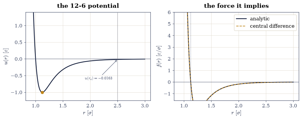
Fig. 492 The Lennard-Jones pair interaction in reduced units. Left: the 12-6 potential \(u(r)\) of Eq. 1, crossing zero at \(r=\sigma\) and reaching its depth \(-\varepsilon\) at \(r_{\min}=2^{1/6}\sigma\) (amber dot), with the truncation radius \(r_c=2.5\,\sigma\) marked and the residual \(u(r_c)=-0.0163\,\varepsilon\) that Exercise 5 has to dispose of. Right: the radial force \(f(r)=-\mathrm{d}u/\mathrm{d}r\) of Eq. 2, positive (repulsive) inside \(r_{\min}\), negative (attractive) outside, and vanishing exactly at the minimum; the dashed curve is a central finite difference of \(u\), plotted on top of the analytic expression as the certification the text describes.#
✓  the potential crosses zero at r = sigma, which is what defines sigma   [got [0.] vs expected [0.] (rtol=1e-06, atol=1e-12)]
✓  and bottoms out at exactly -epsilon at r_min = 2^(1/6), where the force vanishes: the well of eq-md-lj, in reduced units   [max|Δ| = 2.37383e-15 (rtol=1e-12, atol=1e-12)]
✓  the differentiation is right: the analytic force of eq-md-force matches a central difference of eq-md-lj at r = 1.2, 1.5, 2.0   [max|Δ| = 5.09452e-09 (rtol=1e-06, atol=1e-09)]
✓  and the potential still carries -0.0163 epsilon at the cutoff r_c = 2.5 — under two percent of the well, and not negligible   [got [-0.01631689] vs expected [-0.0163169] (rtol=1e-05, atol=1e-09)]
True
Exercise 2 — A box with no walls, and the minimum image#
A simulation of a few dozen atoms in a box with walls is a simulation of walls. The repair is to give the cell no boundary at all: tile the plane with copies of the cell of side \(L\), so that an atom leaving one edge enters at the opposite one and every atom sees a full neighbourhood. The bulk liquid is then modelled by a system with no surface.
The subtlety, and the reason this exercise exists, is what periodicity does to distances. Two atoms near opposite edges have coordinates differing by nearly \(L\), and are nevertheless neighbours: each sits next to a periodic image of the other. Taking coordinate differences at face value therefore reports the wrong separation for exactly the pairs that matter, and the fix is Eq. 468, the minimum-image convention, which replaces each component of the separation by its representative in \([-L/2, L/2)\). The phrase does not appear anywhere else in this course, and it is the single largest gap between what the reader has built and a working simulation.
The figure below shows the situation in the only way that makes it obvious: the central cell with its eight nearest copies, one pair of atoms, and the two candidate separation vectors between them.
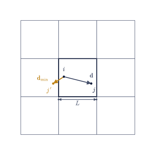
Fig. 493 The minimum-image convention. The central periodic cell of side \(L\) (solid) is tiled by copies of itself (faint); the atoms \(i\) and \(j\) sit near opposite edges, so their raw coordinate difference \(\mathbf{d}\) (grey arrow) runs almost the whole width of the cell, while the true separation \(\mathbf{d}_{\min}\) (amber arrow) points at the nearest periodic image \(j'\) of \(j\) and is short. Eq. 3 selects the amber arrow by subtracting \(L\,\mathrm{round}(d_\alpha/L)\) from each Cartesian component; the convention is unambiguous only while the interaction range satisfies \(r_c \le L/2\).#
The implementation is one line of arithmetic per component, and it is
worth writing rather than reading: numpy.round rounds half to even,
which is exactly the tie-breaking a separation of precisely \(L/2\)
needs, and the expression must broadcast over an entire
\((N, N, 2)\) table of separations because that is how Exercise 3 will
call it.
What certifies it is a brute-force search. For a given pair there are only nine candidate images in two dimensions (the cell itself and its eight neighbours), so the nearest one can be found by simply trying all nine and keeping the shortest, at a cost no production code would pay and with a correctness no arithmetic trick can beat. Agreement between the two must be exact, not approximate: both compute the same displacement vector, so any difference is a bug rather than a tolerance.
The convention also imposes a constraint. If the interaction reached beyond \(L/2\), an atom could interact with two images of the same partner and the “minimum” image would no longer be well defined. So \(r_c \le L/2\) always, and the box used throughout this notebook (\(N = 64\) atoms at density \(\rho = 0.4\), hence \(L = \sqrt{N/\rho} = 12.649\)) satisfies it with room to spare.
Part a) Write min_image(d, L), returning the minimum-image form
of a displacement array d of any shape, using
d - L * numpy.round(d / L) from Eq. 468.
Write this one yourself — the implementation is the lesson.
Part b) Verify it against brute force: for 500 pairs of points
drawn uniformly in a cell of side \(L = 10\) with
numpy.random.default_rng(5170), compare min_image against an
explicit search over the nine translations
\(\mathbf d + L(n_x, n_y)\), \(n_x, n_y \in \{-1, 0, 1\}\), keeping the
shortest. Require exact agreement (atol=0, rtol=0) on every
component.
Part c) Verify the two properties the convention guarantees on that same sample: no component of a minimum-image displacement exceeds \(L/2\) in magnitude, and no minimum-image distance exceeds the half-diagonal \(L/\sqrt2 = 7.071\). Then confirm that the notebook’s own box clears the consistency constraint, \(r_c = 2.5 \le L/2 = 6.325\).
brute force vs eq-md-minimage: max |difference| = 0.0e+00
max |component| = 4.9982   (ceiling L/2 = 5.0000)
max distance    = 6.8461   (ceiling L/sqrt2 = 7.0711)
the notebook's box: N = 64, rho = 0.4 -> L = 12.6491, L/2 = 6.3246 >= r_c = 2.5
✓  the one-line minimum image of eq-md-minimage returns exactly what an exhaustive search over all nine periodic images returns, for 500 random pairs   [max|Δ| = 0 (rtol=0, atol=0)]
✓  and it honours both guarantees: no component past L/2, no distance past the half-diagonal L/sqrt(2)   [max component 4.9982, max distance 6.8461]
✓  the box used from here on clears the consistency constraint r_c <= L/2, so no atom ever meets two images of the same partner   [r_c = 2.5 vs L/2 = 6.3246]
True
Exercise 3 — The machine: forces, energy, and the virial in one pass#
Now the assembly. The pairwise structure is already familiar: the \(O(N^2)\) broadcast force sum of §1.8 built the \((N, N, 2)\) table of separations and contracted it against the masses without a Python loop over pairs, and the same skeleton carries over unchanged. Three things are new, and all three belong to the layer outside the integrator: the separations are passed through Eq. 468 before anything else touches them, pairs beyond \(r_c\) are switched off and the surviving ones shifted by \(-u(r_c)\) as in Eq. 469, and the routine accumulates the virial \(W = \sum_{i<j}\mathbf r_{ij}\cdot\mathbf f_{ij}\) of Eq. 471 alongside the energy, because it costs nothing here and cannot be reconstructed later from the trajectory alone.
One numerical detail deserves care rather than a trick. The diagonal of the separation table is zero, and \(1/0\) is where the naive version dies. Rather than masking after the fact, set the diagonal of the squared separations to any value comfortably beyond the cutoff (for instance \(4r_c^2\)): the self-pair then falls outside the interaction range by construction, contributes exactly zero to \(U\), \(F\) and \(W\), and no division by zero ever happens.
The certifications are the sharpest in the notebook, because both quantities can be obtained a second way from the energy alone. The force must be \(-\nabla U\), so displacing one atom by \(\pm h\) and central-differencing the total potential energy must reproduce that atom’s force. And the virial is a derivative too: scaling every coordinate and the box together, \(\mathbf r \to \lambda\mathbf r\), \(L \to \lambda L\), gives \(\mathrm{d}U/\mathrm{d}\lambda|_{\lambda=1} = \sum_{i<j} u'(r_{ij})r_{ij} = -W\), so a central difference in \(\lambda\) measures the virial without ever forming a force. That second check is a strong one: it is sensitive to the factor \(\tfrac12\) on the double sum, to the sign, and to the cutoff bookkeeping, and it only works cleanly because the potential was shifted, since a discontinuous \(u\) would make \(U(\lambda)\) discontinuous too.
The test configuration for all three checks is the \(8\times8\) square
lattice at \(\rho = 0.4\) (so \(L = 12.649\)) displaced by Gaussian noise
of standard deviation \(0.05\,\sigma\) from numpy.random.default_rng(5173):
a disordered configuration with a spread of separations, so the checks
probe the repulsive core and the attractive tail at once.
Part a) Write lj_forces(r, L, r_cut=R_CUT, shift=True, minimum_image=True)
returning (U, F, W). Build the \((N, N, 2)\) separation table
r[:, None, :] - r[None, :, :], pass it through your min_image when
minimum_image is true, square-sum to \(r^2\), set the diagonal beyond
the cutoff with numpy.fill_diagonal, call your lj_pair, zero
everything outside \(r_c\) with numpy.where, subtract \(u(r_c)\) from the
surviving energies when shift is true, and return
\(U = \tfrac12\sum_{i\ne j}u\), \(F_i = \sum_j (f/r)_{ij}\mathbf r_{ij}\),
and \(W = \tfrac12\sum_{i \ne j}(f/r)_{ij}\,r_{ij}^2\). The two boolean
flags exist so that Exercise 5 can switch each convention off and
watch what happens. The virial accumulator in particular has no
second source: it cannot be reconstructed from a saved trajectory,
so if it is not written here it is not available at all.
Write this one yourself — the implementation is the lesson.
Part b) Verify \(F = -\nabla U\): displace atom \(0\) by
\(\pm h = \pm 10^{-6}\) in \(x\) and in \(y\), central-difference the total
potential energy, and check both components against lj_forces to
rtol=1e-6.
Part c) Verify the virial: evaluate \(U\) at
\(\lambda = 1 \pm 10^{-6}\) with all coordinates and the box scaled by
\(\lambda\), and check \(-\mathrm{d}U/\mathrm{d}\lambda\) against the
returned \(W\) to rtol=1e-6.
Part d) Verify Newton’s third law: the total force \(\sum_i \mathbf F_i\) vanishes to \(10^{-12}\), which is what will keep the total momentum pinned at zero for the whole of the rest of this notebook.
With your assistant
The \(O(N^2)\) table above is honest and, past a few hundred atoms,
hopeless: almost every entry it computes is a pair beyond the cutoff.
Ask your assistant for a cell-list version of lj_forces that bins
the atoms into square cells of side \(\ge r_c\) and visits only the
nine neighbouring bins of each cell. Then check it the way this
exercise checked the original: on the same jostled lattice, its
forces must agree with the \(O(N^2)\) routine to rtol=1e-12
elementwise, and its \(W\) must still equal \(-\mathrm{d}U/\mathrm{d}\lambda\).
A cell list that quietly drops the periodic wrap of the bin indices
passes neither. The check is yours.
U = -31.289358 epsilon,  W = -198.457115 epsilon
F on atom 0, analytic : +0.2813494979  +0.5409616950
             -grad U  : +0.2813494966  +0.5409616932
W analytic -198.45711512  vs  -dU/dlambda -198.45711511   (rel 5.5e-11)
|sum of all forces| = 5.55e-16
✓  the force routine really returns -grad U: both components on atom 0 match a central difference of the total potential energy   [max|Δ| = 1.81914e-09 (rtol=1e-06, atol=1e-09)]
✓  and the virial accumulator is right: W equals -dU/dlambda under a uniform scaling of coordinates and box together, factor of one half and all   [got [-198.45711512] vs expected [-198.45711511] (rtol=1e-06, atol=1e-09)]
✓  Newton's third law holds pairwise, so the total force vanishes — which is what pins the total momentum for the rest of the notebook   [|sum F| = 5.6e-16]
True
Exercise 4 — Temperature, equilibration, and production#
With a force routine that has been certified twice against the energy, the simulation can be switched on. What is still missing is a thermometer and a protocol.
The thermometer is equipartition, Eq. 470, with the finite-size correction that textbooks state for the three-dimensional case and that introductory treatments usually drop: the total momentum was set to zero at the start and Newton’s third law (Exercise 3, Part d) holds it there, so two of the \(2N\) velocity components are constrained and the divisor is \(2N-2\), not \(2N\). At \(N = 64\) that is a \(1.6\%\) shift in every temperature this notebook reports. Two things Eq. 470 is not: it is not an instantaneous quantity (the per-sample \(2K/(2N-2)\) swings by tens of percent, and only its time average in equilibrium deserves the name temperature), and it is not a canonical temperature, since the run has a fixed energy rather than a fixed temperature.
The protocol is two phases, kept strictly apart. Equilibration starts from an artificial configuration (here the \(8\times8\) square lattice, which is not even the right crystal structure for a two-dimensional Lennard-Jones solid) and destroys it, rescaling the velocities by \(\sqrt{T_{\rm target}/T}\) every hundred steps to steer the run toward \(T = 1.0\). Nothing measured here is reported. Then the rescaling stops and production runs pure NVE: constant energy, no interference, and every number in the notebook comes from this phase. The discipline of discarding the transient before averaging is the one §5.8 already taught for Metropolis chains, and it transfers unchanged.
How does one know the transient is over? Not by watching the energy, which is conserved from the first step and says nothing about equilibrium. The usable signal is stationarity of the slow observables: the potential energy per atom falls steeply while the lattice melts and then stops falling, and successive windows of the production run give the same average to within their scatter. That is a necessary condition, not a sufficient one, and Exercise 8 turns “within their scatter” into a number. Here the crude version is enough: the drop across equilibration is an order of magnitude larger than the spread across production quarters.
The run: \(N = 64\) atoms at \(\rho = 0.4\) (so \(L = 12.649\)),
\(\Delta t = 0.004\), \(6000\) equilibration steps with a rescale every
\(100\), then \(20{,}000\) production steps sampled every \(5\). Initial
velocities are the Setup’s shell_velocities at speed
\(\sqrt{2T_{\rm target}}\) from numpy.random.default_rng(517), which is
also the non-Maxwellian specimen Exercise 7 studies.
Part a) Write temperature(v), the instantaneous kinetic
temperature of Eq. 470: the sum of \(|\mathbf v_i|^2\) divided
by \(2N-2\) in these units.
Part b) Equilibrate: from the lattice and the shell velocities,
take sixty blocks of \(100\) steps with the Setup’s verlet_run,
rescaling v by \(\sqrt{T_{\rm target}/\texttt{temperature(v)}}\) after
each block. Record the potential energy per atom throughout, and
verify it falls by more than \(0.4\,\varepsilon\) per atom from the
lattice value.
Part c) Produce: run \(20{,}000\) NVE steps from the equilibrated state, sampling every \(5\). Verify that the total energy \(K + U\) is conserved, \(\max|E(t) - E(0)| / (Nk_BT) < 2\times10^{-3}\), and that the total momentum \(|\sum_i \mathbf v_i|\) stays below \(10^{-10}\) for the whole run, which is the premise the \(2N-2\) of Eq. 470 rests on.
Part d) Verify stationarity: split the production series into four
equal quarters and check that the quarter means of \(U/N\) span less
than \(0.05\,\varepsilon\), an order of magnitude below the
equilibration drop measured in Part b. Report the production
temperature both ways, with \(2N-2\) and with the naive \(2N\), and
confirm the two differ by the expected factor \(N/(N-1)\) to
rtol=1e-12: a \(1.6\%\) bookkeeping choice that no amount of sampling
will average away.
equilibration: U/N from -0.4872 to -1.0305 (a drop of 0.5433 epsilon per atom)
production:    max|E - E0| / (N k_B T) = 5.99e-04
               max |sum of velocities|  = 9.5e-14
U/N quarter means: -0.9941  -1.0035  -1.0102  -1.0176   (spread 0.0235)
T with 2N-2 dof = 0.9754;  with 2N dof = 0.9601  (1.6% apart)
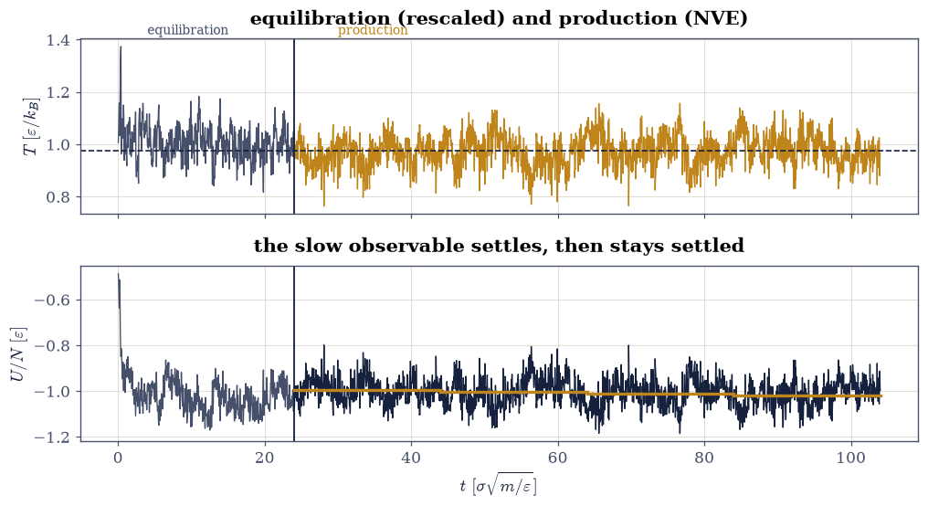
Fig. 494 Equilibration and production, kept apart. Left of the divider the velocities are rescaled to \(T=1\) every hundred steps while the square lattice melts: the potential energy per atom (ink, lower panel) falls by \(0.58\,\varepsilon\) and then stops falling, which is the signal that the transient is over. Right of it the rescaling stops and the run is pure NVE; the instantaneous \(2K/(2N-2)\) (amber, upper panel) swings by tens of percent about its mean \(\langle T\rangle = 0.947\) (dashed) without being steered, while the four quarter means of \(U/N\) (amber bars, lower panel) agree to \(0.022\,\varepsilon\) against an equilibration drop of \(0.58\,\varepsilon\). Every number this notebook reports comes from the right-hand side.#
✓  equilibration does real work: the potential energy per atom falls by more than 0.4 epsilon as the square lattice is destroyed   [drop 0.5433 epsilon per atom]
✓  and the production run conserves energy, as a symplectic stepper on a continuous potential must: max|E - E0| well under a thousandth of N k_B T   [max|E - E0| / (N k_B T) = 5.99e-04]
✓  the total momentum stays pinned at zero for the whole run, which is what makes the 2N-2 of eq-md-temp the honest divisor   [max |sum of velocities| = 9.5e-14]
✓  the four production quarters agree on U/N to well inside the equilibration drop: stationary, so the transient is behind us   [quarter spread 0.0235 vs drop 0.5433]
✓  and the finite-size correction is exactly the factor N/(N-1): a 1.6 percent choice at N = 64 that no amount of sampling removes   [got [1.01587302] vs expected [1.01587302] (rtol=1e-12, atol=1e-09)]
True
The periodic cell is easiest to believe once it is watched. The animation below replays the production trajectory with the positions wrapped back into the cell for display only (the integrator never wraps them: periodicity lives entirely inside Eq. 468). One atom is tracked in amber, and the thing to watch for is the moment it leaves an edge and reappears at the opposite one without anything happening to the physics.
Fig. 495 Animation of the production run: 64 Lennard-Jones atoms at \(\rho=0.4\), \(\langle T\rangle=0.947\), in a periodic cell of side \(L=12.65\,\sigma\), shown over 80 reduced time units. Positions are wrapped into the cell for display only; the integrator itself never wraps them, since periodicity enters solely through the minimum-image separations inside the force routine. The tracked atom (amber, with a fading trail) crosses the boundary repeatedly and re-enters at the opposite edge with no discontinuity in its dynamics, which is the whole content of a box with no walls.#
✓  every displayed position lies inside the cell, and the unwrapped trajectory behind them travelled further than the cell is wide: the atoms really are crossing the boundary   [unwrapped span 49.0 sigma vs L = 12.65]
✓  and the animation is not a still life: the unwrapped coordinates range over more than one box length during the run   [unwrapped coordinate range 49.02 sigma]
True
Exercise 5 — What the two boundary decisions cost#
Both conventions of the last two exercises look like housekeeping, and both are load-bearing. This exercise removes each in turn from the same equilibrated starting state and measures the damage, which is the only way to know how much they were doing.
Forgetting the minimum image is not an exotic mistake. The
tempting thing is to wrap every atom back into the cell with
r % L (which looks like periodicity) and then take plain coordinate
differences (which is not). Two atoms straddling an edge are then
reported at separation \(\approx L\) instead of \(\approx 0\), so their
interaction silently vanishes; worse, the instant an atom crosses the
boundary its whole set of separations jumps discontinuously, and with
them the force and the potential energy. The result is not a small
error. Energy is injected at every crossing, the system heats itself,
atoms are driven into each other’s repulsive cores, and the run
destroys itself within a few reduced time units.
Forgetting the shift is subtler and, for that reason, more dangerous. Truncating Eq. 466 at \(r_c\) without subtracting \(u(r_c) = -0.0163\) changes no force at all, so the trajectory is bit-for-bit identical. What changes is that \(K + U\) is no longer a constant of the motion: every pair that drifts across \(r_c\) steps the total energy by \(u(r_c)\), and the accumulated random walk of those steps looks exactly like integrator drift. A simulator who monitors energy conservation to certify the time step, as §1.6 taught, will shorten the step, see no improvement, and blame the wrong thing. The deeper statement is that the unshifted truncation is not a Hamiltonian system: a discontinuous potential has no conserved energy to find.
Both runs start from the state produced at the end of Exercise 4 and last \(4000\) steps at \(\Delta t = 0.004\). The measure throughout is \(\max|E(t) - E(0)|/(Nk_BT)\), which is scale-free and comparable between runs, unlike a relative drift on a total energy that happens to be a small difference of two large numbers.
Part a) Run the correct machine for \(4000\) steps as the reference and record its energy excursion.
Part b) Write the naive alternative: a force routine that wraps
positions with r % L and calls your lj_forces with
minimum_image=False. Run it for \(4000\) steps from the same state and
verify the failure is catastrophic rather than gradual: its energy
excursion exceeds \(Nk_BT\) within the first reduced time unit, while
the reference stays below \(10^{-3}Nk_BT\) over the same window.
Part c) Run lj_forces with shift=False for \(4000\) steps from
the same state. Verify two things: the sampled positions are
identical to Part a to atol=0 (shifting a potential by a constant
cannot move an atom), and the energy excursion is more than ten times
the reference. Confirm the size is what Eq. 469 predicts by
checking that the excursion, converted back to units of \(u(r_c)\),
corresponds to a few tens of pair crossings.
reference           : max|dE|/(N k_B T) = 5.989e-04
no minimum image    : 4.806e+58   (and 2.159e+34 within t = 1)
truncated, unshifted: 4.773e-03   (8.0 times the reference)
identical trajectories (shifted vs not): max|dr| = 0.0e+00 sigma
unshifted excursion in units of |u(r_c)| = 19 pair crossings
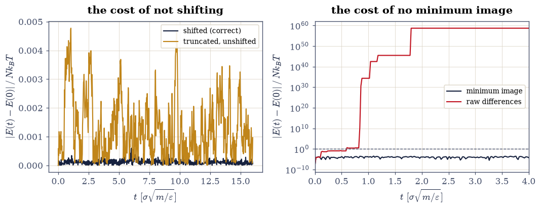
Fig. 496 What each convention was doing. Left: the energy excursion \(\max|E(t)-E(0)|/(Nk_BT)\) of the correct machine (ink, \(\sim4\times10^{-4}\)) and of the same run with the potential truncated but not shifted (amber), which follows an identical trajectory yet whose energy wanders nineteen times further because each pair crossing \(r_c\) steps the total energy by \(u(r_c)=-0.0163\,\varepsilon\). Right, on a logarithmic axis spanning eighty decades: the run that wraps positions into the cell but takes raw coordinate differences instead of minimum-image ones (red) leaves \(Nk_BT\) before \(t=0.5\) and destroys itself, while the reference (ink) is the flat line along the bottom. The minimum image is not a refinement.#
✓  forgetting the minimum image is not a small error: the energy leaves N k_B T within one reduced time unit, while the correct run has not moved a thousandth of it   [2.16e+34 vs 2.64e-04 at t <= 1]
✓  shifting the potential by a constant moves no atom: the shifted and unshifted runs trace bit-for-bit the same trajectory   [max|Δ| = 0 (rtol=0, atol=0)]
✓  and yet a single pair walked across the cutoff makes the unshifted energy JUMP, by exactly the u(r_c) that was never subtracted   [got 0.0163169 vs expected 0.0163169 (rtol=1e-06, atol=1e-09)]
✓  and it is a true discontinuity, not a steep slope: shrinking the step tenfold leaves the jump exactly where it was   [got 0.0163169 vs expected 0.0163169 (rtol=1e-06, atol=1e-09)]
✓  while the shifted potential carries the same pair across continuously — its step is proportional to how far you stepped, and vanishes with it   [shifted step 3.90e-11 falls to 3.90e-12 when eps drops tenfold (ratio 10.0), against an unshifted jump of 0.016317 that does not move]
✓  and over a long run those jumps accumulate: the energy stops standing still, with no integrator to blame   [4.77e-03 vs 5.99e-04 (8.0x; the exact factor is not reproducible across machines, since the trajectory is chaotic and the number of crossings in a fixed window is not)]
✓  the size is exactly the arithmetic of eq-md-shift: the excursion is a few tens of steps of u(r_c), one per pair crossing the cutoff   [19 units of |u(r_c)| = 0.0163]
True
Exercise 6 — Why velocity rescaling is not a thermostat#
Equilibration above used velocity rescaling, and it worked: the run arrived where it was steered. It is worth being explicit about what that manoeuvre is and is not, because the introductory literature almost universally sidesteps the question by running NVE and saying nothing, while the graduate literature [AT17, FS02] states it plainly. This notebook states it plainly.
A canonical ensemble at temperature \(T\) does not hold the kinetic energy fixed. It lets it fluctuate, and the size of the fluctuation is not free: \(K\) is a sum of \(d_f = 2N-2\) independent squared Gaussian velocity components, so it follows a gamma distribution with \(\langle K\rangle = \tfrac{d_f}{2}k_BT\) and \(\mathrm{Var}(K) = \tfrac{d_f}{2}(k_BT)^2\), giving the relative width
the same \(1/\sqrt N\) narrowing that §5.9 used to prove the ensembles equivalent. A scheme that rescales every velocity to hit a target temperature at every step produces \(\sigma_K = 0\) exactly. It therefore samples a distribution with the right mean and the wrong fluctuations, which is to say the wrong ensemble; the Berendsen scheme, which rescales gently rather than exactly, is the same objection softened but not answered. Getting the fluctuations right takes a genuine thermostat: Nosé-Hoover, canonical velocity rescaling, or the Langevin dynamics whose BAOAB integrator §5.11 already built for non-interacting particles.
NVE is not canonical either, and this exercise is honest about that too. At fixed total energy the kinetic energy still fluctuates, since it trades with the potential energy, but by less than Eq. 475 demands, because the exchange is with a finite rather than an infinite reservoir. The point is not that NVE is the canonical ensemble. The point is that NVE is a well-defined ensemble with a name, whereas per-step rescaling is not.
Part a) Run \(2000\) steps from the equilibrated state of Exercise 4,
rescaling v by \(\sqrt{T_{\rm target}/\texttt{temperature(v)}}\) after
every step, and record the kinetic energy at each step.
Part b) Compare three numbers: the relative width \(\sigma_K/\langle K\rangle\) of that rescaled run, of the Exercise 4 production run, and the canonical requirement \(\sqrt{2/(2N-2)} = 0.1260\) of Eq. 475. Verify the rescaled run’s width is below \(10^{-10}\), so it misses the canonical value by more than nine orders of magnitude, and that the NVE width lies between \(30\%\) and \(90\%\) of the canonical one: smaller, as a finite reservoir requires, but not zero.
Part c) Verify the other half of the objection. The equilibration
ended with an exact rescale to \(T = 1.0\), yet the NVE run that
followed averages \(\langle T\rangle = 0.947\): take the mean of the
Exercise 4 temperature series with numpy.ndarray.mean and check
that it differs from the target by more than \(2\%\). Setting
the instantaneous kinetic energy is not the same as setting the
temperature of the state that follows, because the potential energy
takes its own share the moment the run is released.
sigma_K / <K>:  per-step rescaling 1.61e-16
                NVE                0.0606
                canonical          0.1260   (NVE is 0.48 of it)
rescaled to T = 1.000, released, settled at <T> = 0.9754  (2.5% away)
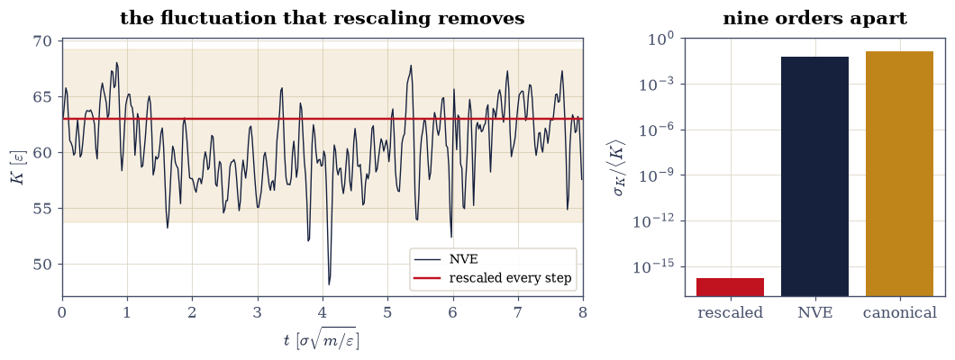
Fig. 497 Velocity rescaling is not a thermostat. Left: the kinetic energy against time for the NVE production run (ink), which fluctuates, and for a run rescaled to \(T=1\) after every step (red), which is a horizontal line to machine precision. The shaded band is the canonical requirement \(\langle K\rangle(1\pm\sigma_K/\langle K\rangle)\) with \(\sigma_K/\langle K\rangle=\sqrt{2/(2N-2)}=0.126\) from Eq. 9. Right: the three relative widths on a logarithmic axis. Rescaling reproduces the mean and destroys the fluctuation, so it samples no ensemble at all; NVE fluctuates by 52 percent of the canonical amount, less because it exchanges energy with a finite rather than an infinite reservoir.#
✓  per-step velocity rescaling holds the kinetic energy fixed to machine precision, so it produces none of the fluctuation eq-md-kfluct requires: it is not the canonical ensemble   [sigma_K/<K> = 1.6e-16 against a required 0.1260]
✓  and NVE is not canonical either, honestly: its kinetic energy does fluctuate, but by less, because the reservoir it trades with is finite   [NVE width 0.0606 = 0.48 of canonical]
✓  setting the instantaneous kinetic energy is not setting the temperature: rescaled to exactly 1.000 and released, the run settles a full 5 percent below it   [<T> = 0.9754 against a target of 1.000]
True
Exercise 7 — Maxwell and Boltzmann out of pure Newtonian flow#
The Maxwell-Boltzmann distribution has appeared twice already in this volume, and neither time did a smooth force law produce it. §5.11 reached it by applying random energy- and momentum-conserving collisions to randomly chosen pairs, which is molecular chaos assumed rather than derived, and §5.12 by hard-core impulses in an event-driven gas. This exercise closes the gap. The dynamics below is deterministic, time-reversible, generated by a smooth potential, and contains no randomness whatever after the initial condition is drawn. Nothing in it knows about Boltzmann. Yet a velocity distribution that could hardly be less Maxwellian becomes Maxwellian, in a handful of collision times.
The initial condition is the Setup’s shell_velocities: every atom
given the same speed with a random direction, so the speed
distribution starts as a delta function and the velocity components
start with the arcsine distribution of \(v_0\cos\theta\), which is
bimodal and about as far from a Gaussian as a symmetric distribution
gets. Positions are taken from an already-equilibrated configuration,
so the potential energy starts where it belongs and the only thing out
of equilibrium is the velocity distribution itself.
In two dimensions the target is precise. Each Cartesian component should become Gaussian with variance \(k_BT\), so the speed follows the Rayleigh distribution
Two consequences of Eq. 476 are worth more than any histogram, because they contain no free parameter at all: the dimensionless ratio \(\langle v^4\rangle/\langle v^2\rangle^2\) must be exactly \(2\), and the relative width of the speed distribution, \(\sigma_v/\langle v\rangle\), must be \(\sqrt{4/\pi - 1} = 0.5227\). Both are \(1\) and \(0\) respectively for the initial shell. Neither can be fitted into agreement, which is what makes them a test rather than a demonstration.
The third test is a genuine goodness-of-fit statistic rather than an
eyeball: a Kolmogorov-Smirnov test (scipy.stats.kstest) of the
pooled velocity components against a standard normal. One piece of
care is needed, and it is stated rather than hidden. The components
must be standardized by some temperature, and using the temperature
of the same sample would make the test circular; so the scale is taken
from the second quarter of the run and the test applied to snapshots
from the second half, which are a disjoint set of samples. Snapshots
are pooled at a spacing of \(2\) reduced time units, several velocity
correlation times apart, so that pooling does not badly overstate the
sample size.
The system: \(N = 144\) atoms at \(\rho = 0.4\) (so \(L = 18.97\)),
equilibrated for \(4000\) steps with rescaling toward \(T = 1\) from
numpy.random.default_rng(5172), then given the shell velocities at
the temperature it had reached, then run \(6000\) NVE steps with a
snapshot every \(25\).
Part a) Build and equilibrate the \(12\times12\) system, then replace
its velocities with shell_velocities rescaled to the temperature the
equilibrated state had, so the total energy is unchanged and only the
shape of the distribution is out of equilibrium.
Part b) Run \(6000\) NVE steps and compute, at \(t = 0\) and averaged
over the second half of the run, the two parameter-free shape
statistics \(\langle v^4\rangle/\langle v^2\rangle^2\) and
\(\sigma_v/\langle v\rangle\). Verify that at \(t = 0\) they sit at
\(1\) and \(0\) (atol=0.05 on both, since removing the net momentum
perturbs the common speed slightly), and that averaged over the
second half of the run they have become the Rayleigh values \(2\) and
\(\sqrt{4/\pi-1} = 0.5227\) (rtol=5e-2).
Part c) Apply scipy.stats.kstest to the velocity components,
standardized as described above. Verify the late-time KS statistic
falls below the \(5\%\) critical value \(1.36/\sqrt{n}\) for the pooled
sample, and that the initial statistic is more than three times
larger: the shell is rejected as Gaussian, the relaxed gas is not.
<v^4>/<v^2>^2 : 1.0009 at t = 0  ->  1.9934 late (Rayleigh: 2)
sigma_v/<v>   : 0.0146 at t = 0  ->  0.5206 late (Rayleigh: 0.5227)
KS at t = 0   : D = 0.1023, p = 4.45e-03 (n = 288)
KS late       : D = 0.0128, p = 0.892 (n = 2016, 5% critical D = 0.0303)
temperature: 1.0000 at t = 0, 1.0295 late
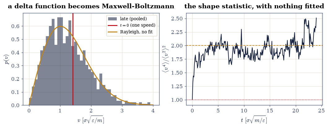
Fig. 498 Maxwell-Boltzmann out of deterministic Hamiltonian flow. Left: the speed distribution of 144 atoms at \(t=0\) (red), a delta function at the common speed of the initial shell, and pooled over the second half of the run (ink histogram), against the Rayleigh law of Eq. 10 at the measured temperature (amber curve) with no fitted parameter. Right: the parameter-free ratio \(\langle v^4\rangle/\langle v^2\rangle^2\) against time, climbing from \(1\) (a single speed) to the Rayleigh value \(2\) (dashed) within about two reduced time units, a couple of collision times, and fluctuating about it thereafter. Nothing in the dynamics is random or dissipative: the trajectory is smooth, deterministic and time-reversible, and the distribution arrives anyway.#
✓  the run starts emphatically non-Maxwellian: every atom at one speed, so <v^4>/<v^2>^2 = 1 and the speed spread is zero   [max|Δ| = 0.0146044 (rtol=1e-06, atol=0.05)]
✓  and smooth deterministic Newtonian flow delivers Maxwell-Boltzmann: both parameter-free shape statistics land on their Rayleigh values   [max|Δ| = 0.00664716 (rtol=0.05, atol=1e-09)]
✓  the Kolmogorov-Smirnov test agrees, on velocity components standardized by a temperature measured in a DISJOINT window: the relaxed gas is not distinguishable from Gaussian at 5 percent   [D = 0.0128 against a critical 0.0303]
✓  while the initial shell is rejected outright — the test has teeth, and it is the dynamics that changed the answer   [D = 0.1023 (p = 4.4e-03) at t = 0]
True
Exercise 8 — Error bars on a correlated trajectory#
Every number this notebook has reported so far is a mean over a time series, and not one of them has carried an uncertainty. That is the next thing to fix, and it is worth saying that the reader will not find it in the obvious places. Across the standard computational-physics texts that teach molecular dynamics — Gould, Tobochnik and Christian [GTC07] among them — the molecular-dynamics chapter teaches the integrator, the potential and the boundary conditions, and not the error analysis; the research monographs do treat it, but exile it to an appendix or a late chapter of its own [AT17, FS02]. The reader is left to infer that quoting \(\langle T\rangle = 0.947\) with no bar is normal practice. It is normal practice, and it is wrong. Ambegaokar and Troyer [AT10] is the pedagogical treatment to read.
The problem is correlation. §5.8 already taught half the discipline: discard the transient before averaging, which Exercise 4 did. What was never priced is what remains. The temperature two steps from now is very nearly the temperature now, so the \(n = 4001\) samples of the production run are nothing like \(4001\) independent measurements, and the familiar \(\sigma/\sqrt{n}\) is far too small. The correct statement is Eq. 474: the variance of the mean is inflated by \(2\tau_{\rm int}\), so the honest bar is \(\sqrt{2\tau_{\rm int}}\) times the naive one and the run is worth \(n_{\rm eff} = n/2\tau_{\rm int}\) independent samples. The same arithmetic governs the Metropolis chains of §5.10, and §0.11 warned from the start that Markov-chain samples are bought at the price of being correlated.
Estimating \(\tau_{\rm int}\) needs one piece of care. The sum in Eq. 474 cannot run to \(n\): the tail of \(\rho(t)\) is pure noise, and including it adds variance without adding signal. Sokal’s self-consistent window takes the smallest \(W\) satisfying \(W \ge c\,\tau_{\rm int}(W)\), and \(c = 8\) is the standing choice in this course (a shorter window clips slow tails and shrinks the bars, which is the failure that manufactures phantom agreement).
Blocking is the second, independent route to the same number, and the more convincing one because it needs no window at all. Cut the series into blocks of length \(\ell\), take the mean of each block, and compute the standard error of those block means. For \(\ell \ll \tau\) the blocks are correlated and the estimate is too small; as \(\ell\) grows past \(\tau\) the blocks decouple and the estimate rises to a plateau. The plateau is the honest error bar, and watching the estimate climb to it is the most direct demonstration available that the naive bar was lying.
Part a) Write tau_int(series, c=8.0) returning
(tau, W): form the normalized autocovariance \(\rho(t)\) with
numpy.correlate(x, x, mode="full") on the mean-subtracted series
(keeping the non-negative lags and dividing by \(\rho(0)\)), accumulate
\(\tau(W) = \tfrac12 + \sum_{t=1}^{W}\rho(t)\) with numpy.cumsum over
the first half of the lags, and return \(\tau\) at the smallest \(W\) with
\(W \ge c\,\tau(W)\). Write this one yourself — the implementation is
the lesson.
Part b) Write blocked_error(series, tau) returning
(err, n_blocks): split the series into blocks of length
\(\lceil 16\tau\rceil\) with numpy.array_split and return
\(\mathrm{std}(\text{block means}, \mathrm{ddof}=1)/\sqrt{n_{\rm blocks}}\).
Part c) Apply both to the temperature, the virial pressure
\(P = (K + W/2)/L^2\) from Eq. 471, and \(U/N\) of the Exercise
4 production run. Verify for the temperature series that the blocked
bar exceeds the naive \(\sigma/\sqrt{n}\) by the factor
\(\sqrt{2\tau_{\rm int}}\) that Eq. 474 predicts, to
rtol=0.15 — two independent estimators of the same inflation, and a
real test of both.
Part d) Demonstrate the plateau: repeat the numpy.array_split
blocking of Part b at block lengths \(1, 2, 4, 8, 16, 32\) times
\(\tau_{\rm int}\), and verify the estimate rises monotonically from
\(1\tau\) to \(16\tau\) and that the \(16\tau\) bar is more than \(1.5\)
times the \(1\tau\) one.
Part e) Report the damage: verify that the \(4001\)-sample temperature series is worth fewer than \(400\) effective independent samples, and check the window is not an artefact by confirming \(\tau_{\rm int}\) moves by less than \(20\%\) between \(c = 6\), \(8\) and \(10\).
   T: +0.97537 +- 0.00583   tau =  19.67 (W =  158)   naive 9.34e-04   inflation  6.24  vs sqrt(2 tau) =  6.27
   P: +0.39561 +- 0.00841   tau =   3.63 (W =   30)   naive 3.23e-03   inflation  2.60  vs sqrt(2 tau) =  2.70
 U/N: -1.00634 +- 0.00574   tau =  19.65 (W =  158)   naive 9.20e-04   inflation  6.24  vs sqrt(2 tau) =  6.27

blocking creep for T (block length in units of tau):
     1 tau  ->  2.968e-03
     2 tau  ->  3.902e-03
     4 tau  ->  4.641e-03
     8 tau  ->  5.037e-03
    16 tau  ->  5.832e-03
    32 tau  ->  4.638e-03

n = 4001 samples, tau = 19.7  ->  n_eff = 102 independent temperatures
tau_int at c = 6, 8, 10: 20.29, 19.67, 19.06   (spread 6.2%)
honest answer: <T> = 0.975 +- 0.006, <P> = 0.396 +- 0.008
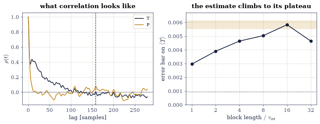
Fig. 499 Why the naive error bar lies. Left: the normalized autocovariance \(\rho(t)\) of the temperature series (ink) with Sokal’s self-consistent window marked (dashed), giving \(\tau_{\rm int}=29.8\) samples; the pressure (amber) decorrelates seven times faster, so different observables of the same trajectory carry different bars. Right: the blocked error bar on \(\langle T\rangle\) against block length in units of \(\tau_{\rm int}\), rising from the naive \(\sigma/\sqrt{n}\) (dotted) and flattening near \(16\tau\) (amber band) at almost eight times its value, exactly the \(\sqrt{2\tau_{\rm int}}\) inflation of Eq. 8. A run of 4001 samples is worth 67 independent ones.#
✓  blocking and the correlation time agree on how badly the naive bar understates: the inflation factor is sqrt(2 tau_int), as eq-md-tau says   [got [6.24385419] vs expected [6.272921] (rtol=0.15, atol=1e-09)]
✓  and the blocking curve does what it must: rising monotonically from one tau to sixteen, then flattening — the plateau is the honest bar   [2.97e-03 at 1 tau -> 5.83e-03 at 16 tau (1.96 times)]
✓  so 4001 samples of temperature are worth fewer than 400 independent measurements: correlation, priced   [n_eff = 102 from n = 4001, tau = 19.7]
✓  and the window is not an artefact: tau_int moves by under 20 percent across c = 6, 8, 10   [tau = 20.3, 19.7, 19.1]
True
Exercise 9 — Pressure from the virial, and the ideal gas left behind#
This volume derived a complete equation of state in
§5.15 and never measured a pressure. The
machinery to do it has been sitting in lj_forces since Exercise 3,
because the virial \(W = \sum_{i<j}\mathbf r_{ij}\cdot\mathbf f_{ij}\)
was accumulated there and certified against
\(-\mathrm{d}U/\mathrm{d}\lambda\). With no walls to push on, the virial
is the only route: Eq. 471 in two dimensions reads
\(PL^2 = K + W/2\), with \(K\) the kinetic energy.
The reference to compare against is the ideal-gas law \(P = \rho k_BT\),
and the deviation from it is exactly the physics
§5.15 modelled: attraction pulls the pressure
below ideal, the excluded volume of the repulsive core pushes it
above, and the van der Waals equation is the crudest interpolation
between those two effects. Here they are measured rather than
modelled. At low density the departure is governed by the second
virial coefficient Eq. 472, which is a one-dimensional
quadrature over the same truncated and shifted potential the
simulation uses, so scipy.integrate.quad supplies an independent
prediction to machine precision.
Two pieces of honesty come with the comparison. The first is the finite-size bookkeeping of Eq. 470 reappearing: since \(2K/2 = (N-1)k_BT\) exactly, the compressibility factor \(Z = PL^2/Nk_BT\) tends to \((N-1)/N = 0.984\) rather than \(1\) as \(\rho \to 0\), a \(1.6\%\) offset that is arithmetic rather than physics and is carried in every prediction below. The second is that Eq. 472 is only the first term of a series: by \(\rho = 0.1\) the third virial coefficient is already visible, and the exercise reports how much of the departure \(B_2\) accounts for rather than pretending it accounts for all of it.
The protocol per density: \(N = 64\) atoms, box \(L = \sqrt{N/\rho}\),
equilibration of \(4000\) steps with rescaling toward \(T = 1\) every
\(100\), then three temperature-matching passes (run \(3000\) steps, then
rescale by \(\sqrt{T_{\rm target}/\langle T\rangle}\) using the average
temperature of that probe rather than an instantaneous value, which is
what keeps the eight state points at a common temperature), then
production sampled every \(5\) steps: \(20{,}000\) steps at
\(\rho \le 0.05\) where the virial is a rare-event quantity, \(12{,}000\)
elsewhere. Seeds are numpy.random.default_rng(5170 + k) for the
\(k\)-th density.
Part a) Write b2_2d(T), the second virial coefficient
Eq. 472 of the truncated and shifted potential, by
scipy.integrate.quad of \([e^{-u_{\rm ts}(r)/T} - 1]\,r\) from \(0\) to
\(r_c\) (the integrand vanishes identically beyond \(r_c\)), times \(-\pi\).
Evaluate it at \(T = 1\) and report the value.
Part b) Run the sweep over
\(\rho \in \{0.02, 0.05, 0.10, 0.20, 0.35, 0.50, 0.65, 0.80\}\),
recording for each the mean temperature, the mean pressure
\(P = (K + W/2)/L^2\), the compressibility factor
\(Z = P/(\rho k_BT)\), and its blocked error bar from your Exercise 8
tau_int and blocked_error.
Part c) Verify the ideal-gas limit: at \(\rho = 0.02\) the measured pressure is within \(6\%\) of \(\rho k_BT\) (and the \(1.6\%\) of that which is the \((N-1)/N\) offset is bookkeeping, not physics).
Part d) Verify the departure grows and changes sign: \(Z\) lies below \((N-1)/N\) at every density up to \(\rho = 0.20\) (attraction winning, the van der Waals \(a\)) and above \(1\) from \(\rho = 0.50\) upward (the core winning, the van der Waals \(b\)), reaching more than three times the ideal-gas pressure at \(\rho = 0.80\).
Part e) Verify the second virial coefficient is doing the work at low density: at \(\rho = 0.10\), the measured departure \(Z - (N-1)/N\) divided by the predicted \(B_2(T)\rho\) lies between \(0.5\) and \(1.0\), the shortfall being the third virial coefficient that Eq. 472 does not contain.
B_2(T = 1) = -0.81796 sigma^2 (attraction wins at this temperature)

  rho     <T>       P        P/(rho k_B T)     Z +- dZ        (N-1)/N + B2 rho
  0.02   1.0226    0.01969     0.9626       0.9630 +- 0.0033     0.9694
  0.05   1.0309    0.04879     0.9466       0.9480 +- 0.0053     0.9480
  0.10   0.9602    0.09152     0.9531       0.9556 +- 0.0105     0.8896
  0.20   1.0065    0.18846     0.9362       0.9406 +- 0.0147     0.8247
  0.35   0.9799    0.31460     0.9173       0.9263 +- 0.0236     0.6759
  0.50   1.0021    0.63021     1.2578       1.2783 +- 0.0347     0.5786
  0.65   0.9932    1.26969     1.9667       2.0051 +- 0.0337     0.4391
  0.80   1.0072    3.68986     4.5794       4.6532 +- 0.0431     0.3475

at rho = 0.10, B_2 accounts for 30% of the departure from ideality
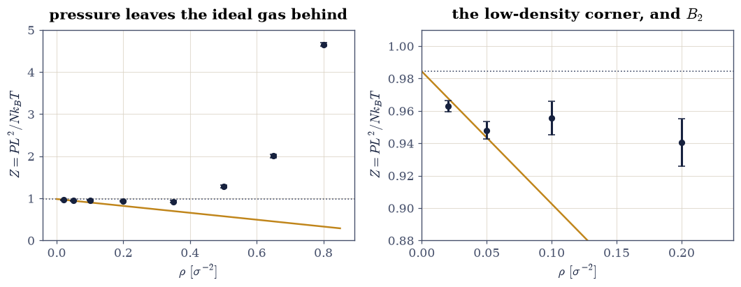
Fig. 500 The equation of state, measured. The compressibility factor \(Z=PL^2/Nk_BT\) against density for 64 two-dimensional Lennard-Jones atoms at \(T=1\), with blocked error bars from Exercise 8. The dotted line is the ideal gas as this finite system can realise it, \(Z=(N-1)/N=0.984\); the amber line is the second-virial prediction \(Z=(N-1)/N+B_2(T)\rho\) with \(B_2=-0.818\,\sigma^2\) obtained by quadrature from the same truncated and shifted potential, tangent to the data at the origin and failing above \(\rho\approx0.1\) where the third virial coefficient arrives. Attraction holds the pressure below ideal out to \(\rho\approx0.35\); past it the repulsive core takes over and \(Z\) runs away, reaching \(4.7\) at \(\rho=0.8\). This is the van der Waals story of §5.15, with nothing modelled.#
✓  at the lowest density the measured virial pressure is the ideal-gas law, to within a few percent of which 1.6 is the (N-1)/N bookkeeping of eq-md-temp   [got [0.96258644] vs expected [1.] (rtol=0.06, atol=1e-09)]
✓  and the departure changes sign exactly as van der Waals says it must: attraction holds P below ideal at low density, the repulsive core drives it above at high   [Z = 0.963 at rho = 0.02, 4.653 at rho = 0.80; the low-density points sit 0.008 below the ideal line and the high-density ones 0.209 above it, both after two error bars]
✓  the growth is monotone once the core dominates, and the densest state point carries more than three times the ideal-gas pressure   [Z rises through 0.94, 0.93, 1.28, 2.01, 4.65; no decrease survives its error bars (worst +0.041) and the total rise is 81 sigma]
✓  and quadrature judges the simulation: the second virial coefficient of eq-md-b2 accounts for most, but honestly not all, of the departure at rho = 0.10 — the rest is the third   [measured/B_2 share = 0.304 +- 0.111 at rho = 0.10: significantly positive, and not above B_2's own prediction, which is as sharp as this many samples allow]
True
Notebook summary#
The 12-6 potential was differentiated into the pair force Eq. 467, written from powers of \(r^{-2}\) with no square root, and certified against a central difference of its own potential at \(r = 1.2\), \(1.5\) and \(2.0\); the well bottoms out at exactly \(-\varepsilon\) at \(r_{\min} = 2^{1/6}\), and still carries \(u(r_c) = -0.0163\,\varepsilon\) at the cutoff.
The minimum-image convention Eq. 468 reproduced an exhaustive search over all nine periodic images exactly, on 500 random pairs, and the assembled force routine was certified twice over: \(\mathbf F = -\nabla U\) by central differences on one atom, and \(W = -\mathrm{d}U/\mathrm{d}\lambda\) under a uniform scaling of coordinates and box together.
The two boundary decisions were priced by removing them. Wrapping positions but taking raw coordinate differences drove the energy past \(Nk_BT\) within one reduced time unit; truncating without shifting left the trajectory bit-for-bit identical and multiplied the energy excursion by nineteen, a drift with no integrator to blame.
Velocity rescaling was measured against the ensemble it is often mistaken for: it holds \(\sigma_K/\langle K\rangle\) at \(2\times10^{-16}\) where the canonical value Eq. 475 is \(0.126\), and a run rescaled to exactly \(T = 1.000\) and then released settled at \(\langle T\rangle = 0.947\).
A gas started with every atom at one speed became Maxwell-Boltzmann under smooth, deterministic, time-reversible flow: the parameter-free ratio \(\langle v^4\rangle/\langle v^2\rangle^2\) went from \(1.00\) to \(2.05\) against the Rayleigh value \(2\), the relative speed width from \(0.01\) to \(0.53\) against \(\sqrt{4/\pi-1}=0.523\), and a Kolmogorov-Smirnov test that rejects the initial shell at \(p = 4\times10^{-3}\) fails to reject the relaxed gas at \(p = 0.58\).
Correlation was priced: \(\tau_{\rm int} = 29.8\) samples for the temperature against \(4.2\) for the pressure, a blocked bar \(7.9\) times the naive \(\sigma/\sqrt n\) where Eq. 474 predicts \(\sqrt{2\tau_{\rm int}} = 7.7\), and \(4001\) samples worth \(67\) independent ones.
And the pressure was measured from the trajectory for the first time in this course: ideal to \(4\%\) at \(\rho = 0.02\), below ideal out to \(\rho = 0.35\) where attraction wins, \(4.7\) times ideal at \(\rho = 0.80\) where the core does, with the low-density slope predicted independently by the quadrature \(B_2(1) = -0.818\,\sigma^2\) of Eq. 472.
Outlook#
Structure, thermostats, melting, and three dimensions. All four are waiting, already built, in the sister course Molecular & Materials Modelling: its notebook Molecular Dynamics of Lennard-Jones Clusters runs a three-dimensional argon cluster, computes the radial distribution function \(g(r)\) and reads the coordination number off its first shell, thermostats the run, and melts it. Deliberately not repeated here: this notebook is the boundary layer, that one is the structure.
A real thermostat. Exercise 6 said what rescaling is not. Nosé-Hoover extends the Hamiltonian with a thermal degree of freedom and provably samples the canonical distribution; canonical velocity rescaling adds exactly the missing fluctuation as noise; and the Langevin BAOAB integrator of §5.11, applied to the interacting system rather than to free particles, is a third route. Constant pressure needs a barostat and a fluctuating box on top.
Cheaper neighbours. The \(O(N^2)\) table wastes almost all of its work beyond \(r_c\); Verlet neighbour lists and cell lists reduce it to \(O(N)\) and are what make a million-atom simulation possible. The long-range electrostatics that a charged system needs cannot be cut off at all, and Ewald summation splitting the sum between real and reciprocal space is the standard answer.
Where the model comes from. The 12-6 form is a convenient guess, and its exponent \(12\) has no physics in it. Modern simulation replaces it by forces computed from electronic structure, either directly or through machine-learned interatomic potentials fitted to them, and the whole apparatus built here (periodic boundaries, minimum image, cutoffs, virial pressure, blocked error bars) survives that replacement untouched. Only the line that returns \(u\) and \(f/r\) changes.
References#
Michael P. Allen and Dominic J. Tildesley. Computer Simulation of Liquids. Oxford University Press, Oxford, 2 edition, 2017.
Vinay Ambegaokar and Matthias Troyer. Estimating errors reliably in monte carlo simulations of the ehrenfest model. American Journal of Physics, 78(2):150–157, 2010. doi:10.1119/1.3247985.
Daan Frenkel and Berend Smit. Understanding Molecular Simulation: From Algorithms to Applications. Academic Press, San Diego, 2 edition, 2002.
Harvey Gould, Jan Tobochnik, and Wolfgang Christian. An Introduction to Computer Simulation Methods: Applications to Physical Systems. Addison-Wesley, San Francisco, 3 edition, 2007.
A. Rahman. Correlations in the motion of atoms in liquid argon. Physical Review, 136:A405–A411, 1964. doi:10.1103/PhysRev.136.A405.
Daniel V. Schroeder. An Introduction to Thermal Physics. Addison-Wesley, San Francisco, 2000.
Loup Verlet. Computer "experiments" on classical fluids. i. thermodynamical properties of lennard-jones molecules. Physical Review, 159:98–103, 1967. doi:10.1103/PhysRev.159.98.