


7.2 Dimensionality Reduction and Farthest-Point Sampling#
Notebook overview#
§7.1 turned an atomic environment into a sixteen-component vector, invariant to everything the energy is invariant to. That solves the representation problem and creates two new ones. Sixteen components cannot be plotted, so there is no way to look at a dataset of environments and see whether it has structure, gaps or duplicates. And a molecular-dynamics run produces environments by the million, of which only a handful can be afforded at the level of theory one actually wants to fit to — so something has to choose.
Both problems have classical answers that predate the machine-learning framing by decades. Principal component analysis finds the directions along which the data varies most and projects onto the first two, which is the standard way to get a picture. Classical multidimensional scaling starts instead from the matrix of pairwise distances and asks for the point set that reproduces them best — a different question, from a different input, which for Euclidean distances turns out to have exactly the same answer, a coincidence worth verifying rather than assuming. Farthest-point sampling greedily picks the point furthest from everything picked so far, which covers the space far more evenly than drawing at random.
The interesting results here are the negative ones. The projection that captures the most variance is not the projection that answers a given question: the leading components here sort environments by coordination and leave the fcc/hcp distinction — the one §7.1 worked hardest to expose — invisible. And farthest-point sampling, asked to cover the space, spends most of its picks on the outliers.
Provenance. This notebook develops Lecture 11 of the course (dimensionality reduction and sampling), an exercise designed by the author (Raymond Amador) to restore a lecture the original exercise set announced but never delivered. Like §7.1 it uses no committed calculation: the ensemble is built here from lattice definitions and thermal displacement. The full course credit is in the footer.
Reading a validation. Each task closes with a check against an independent fact: that a perfect crystal gives a degenerate dataset, that the two projections agree to machine precision, that farthest-point sampling beats random selection at the thing it optimises. A ✗ flags a mismatch; a ✓ is strong evidence, not proof.
Scope. The ensemble is rattled lattices rather than a molecular-dynamics trajectory, so that every environment carries a known label to check the projections against. Both methods here are linear; the nonlinear family (sketch-map [CTP11], t-SNE, UMAP) is left to the Outlook.
Theory in brief#
Principal component analysis#
Collect \(n\) environments as rows of a matrix \(\mathbf Y\), each column centred to zero mean. PCA looks for the direction \(\hat{\mathbf u}\) along which the projected data has the largest variance, then the largest orthogonal to that, and so on. Those directions are the eigenvectors of the covariance matrix \(\mathbf Y^\mathsf{T}\mathbf Y / (n-1)\), and they come directly out of the singular value decomposition
whose right singular vectors (the columns of \(\mathbf V\)) are the principal directions and whose singular values give the variance carried by each, \(\sigma_k^2 / \sum_j \sigma_j^2\). Projecting onto the first two directions is the matrix product \(\mathbf U_{:,:2}\mathbf S_{:2}\). Working from the SVD rather than by forming and diagonalising the covariance matrix is not a stylistic preference: squaring \(\mathbf Y\) squares its condition number, and the small singular values are exactly where that costs accuracy.
Because the columns of a descriptor carry different units and wildly different magnitudes, they are standardised — each divided by its own standard deviation — before any of this. Otherwise PCA reports whichever component happens to be numerically largest, which is a fact about the parametrisation and not about the physics.
Classical multidimensional scaling#
Suppose the coordinates are unavailable and only the matrix of pairwise distances \(d_{ij}\) is known. Classical scaling [Tor52] recovers a point set from them. Double-centring the squared-distance matrix with \(\mathbf J = \mathbf I - \tfrac1n \mathbf{11}^\mathsf{T}\) produces a Gram matrix
whose eigendecomposition \(\mathbf B = \mathbf Q \boldsymbol\Lambda \mathbf Q^\mathsf{T}\) gives the embedding \(\mathbf Q_{:,:m}\boldsymbol\Lambda_{:m}^{1/2}\). When the \(d_{ij}\) are Euclidean distances between points that exist, \(\mathbf B = \mathbf Y\mathbf Y^\mathsf{T}\) exactly, so its eigenvalues are the squared singular values of \(\mathbf Y\) and the two methods return the same embedding up to the sign of each axis. Exercise 3 checks that identity numerically. It matters because the MDS route still works when the “distance” is something a descriptor never produced coordinates for.
Farthest-point sampling#
To choose \(k\) representatives from \(n\) points, start anywhere and repeatedly add the point whose distance to the nearest already-chosen point is largest [IAGiofre+18]. The quantity this minimises, greedily, is the coverage radius: the largest distance from any point of the dataset to its nearest representative. A random subset optimises nothing, and in a dataset with rare regions it will miss them.
Setup#
The Setup below holds this notebook’s instruments — the lattices, the neighbour search, and the descriptor built from scratch in §7.1; restated here as an instrument so this notebook stands alone. The reduction and sampling methods, which are this notebook’s subject, are built in the exercises. It is collapsed so the building stays yours; expand it whenever you want the details.
Exercise 1 — Building an ensemble worth reducing#
Before any projection, the data has to be worth projecting. A perfect crystal is a trap here: every atom of a given phase sits in an environment identical to every other by symmetry, so a dataset of a thousand perfect-crystal environments contains exactly as much information as one of four. Thermal displacement is what makes a real ensemble continuous, and a molecular-dynamics trajectory would supply it; rattling the lattice is the same effect, reproducibly.
Part a) Build the descriptors of many atoms in each perfect lattice and measure the spread within each phase. Establish that the dataset is degenerate.
Part b) Rebuild it with each structure rattled by a Gaussian displacement over a range of amplitudes, and confirm the spread is now non-zero and grows with amplitude. Assemble the full labelled dataset that the rest of the notebook uses.
perfect fcc: largest component-wise standard deviation = 4.64e-14
perfect hcp: largest component-wise standard deviation = 2.66e-14
perfect bcc: largest component-wise standard deviation = 2.01e-14
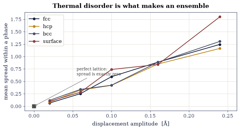
Fig. 81 Spread of the descriptors within each phase, as a function of the amplitude of the Gaussian displacement applied to the atoms. At zero amplitude every atom of a given phase has an environment identical to every other by symmetry, so the spread is exactly zero and a dataset of any size carries no more information than a single point per phase. Thermal displacement is what turns a set of lattices into an ensemble; the spread grows roughly linearly with the displacement, and it is this variation the projections of Exercises 2 and 3 have to organise.#
dataset: 240 environments × 16 descriptor components
classes: fcc (60), hcp (60), bcc (60), surface (60)
mean within-phase spread by amplitude: 0.02 Å -> 0.09, 0.06 Å -> 0.30, 0.10 Å -> 0.54, 0.16 Å -> 0.87, 0.24 Å -> 1.38
Validation 1 — degenerate, then not#
Two checks that bracket the exercise. In the perfect lattices every environment of a phase must be identical to machine precision, which is a consequence of the space-group symmetry and simultaneously a test that the periodic neighbour search is right. Once the structures are rattled the spread must be non-zero and must increase with the displacement, since that is the only thing generating variety in this dataset.
✓  in a perfect lattice every atom of a phase has an identical environment, so the descriptors are equal to machine precision and a larger sample of a perfect crystal contains no more information than a single atom of it   [fcc: 4.6e-14, hcp: 2.7e-14, bcc: 2.0e-14]
✓  while rattling makes the spread non-zero and strictly increasing in the displacement amplitude, which is what turns a handful of lattices into an ensemble with something for a projection to organise   [spread 0.09 < 0.30 < 0.54 < 0.87 < 1.38]
True
Exercise 2 — Principal component analysis#
Sixteen dimensions cannot be looked at. PCA finds the plane in which the data spreads out most and projects onto it, which is the standard first look at any dataset — provided one remembers what it optimises.
Part a) Implement PCA from the singular value decomposition of Eq. 71, returning the projected coordinates and the fraction of the variance carried by each component. Write this one yourself — the implementation is the lesson.
Part b) Project the dataset onto the first two components and colour by phase. Report how much of the variance those two carry.
Part c) Ask what the components actually encode. Correlate each with the displacement amplitude, and measure how far apart the phase centroids are relative to the scatter within a phase. Then check specifically whether fcc and hcp — the pair Eq. 71 knows nothing about, and which §7.1 needed sharp angular functions to separate — are distinguishable in this projection.
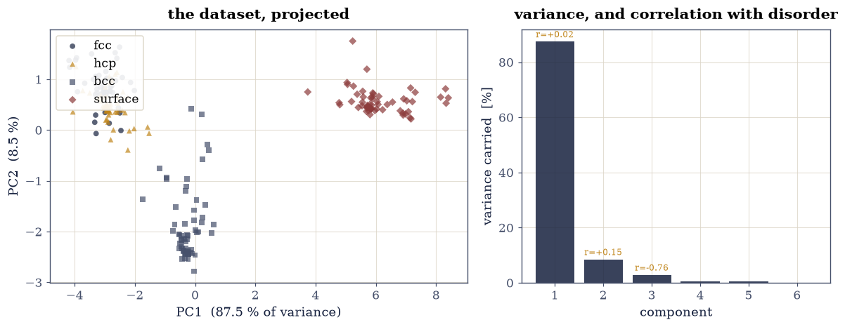
Fig. 82 Left: the environment dataset projected onto its first two principal components, which together carry 96.5 % of the variance. PC1 separates the under-coordinated surface environments from every bulk phase and PC2 separates body-centred cubic from the close-packed pair, but fcc and hcp land on top of each other. Right: the variance carried by each component, with the correlation between that component and the displacement amplitude marked. Disorder is PC3, carrying only about 2 % of the variance — so the projection that shows the most variation is not the one that answers a question about stacking, and would not have been even if more components were plotted.#
PC1 + PC2 carry 96.0 % of the variance
  PC1:  87.5 %   correlation with disorder +0.023   between/within class spread 6.87
  PC2:   8.5 %   correlation with disorder +0.149   between/within class spread 2.70
  PC3:   2.9 %   correlation with disorder -0.762   between/within class spread 0.17

fcc vs hcp centroid gap in the PC1-PC2 plane: 0.99 × the within-class scatter
bcc vs fcc, for comparison:                    9.16 ×
Validation 2 — a good projection, of the wrong thing#
Three checks. The first two components must carry most of the variance, or the picture would be misleading in an ordinary way. The leading component must separate phases rather than track disorder, and disorder must appear only further down the ranking, which is what makes the plot look organised. And the fcc/hcp centroids must sit within roughly one scatter-width of each other while bcc sits far away — the honest statement that this projection has hidden the distinction §7.1 worked to expose.
✓  the first two components carry the great majority of the variance, so the two-dimensional picture is not discarding most of what varies   [PC1 + PC2 = 96.0 %]
✓  the leading component is essentially uncorrelated with the thermal displacement while a later one tracks it closely: PCA has sorted the environments by what they ARE before by how disordered they are, which is why the map looks clean   [|r| with amplitude: PC1 0.02, PC3 0.76]
✓  and yet fcc and hcp overlap in this plane while bcc is far away: the projection that maximises variance is not the projection that answers a question about stacking, and no amount of variance explained would have made it so   [fcc-hcp gap 0.99 × scatter, bcc-fcc gap 9.16 ×]
True
Exercise 3 — The same picture from distances alone#
Classical multidimensional scaling starts from a different input — the matrix of pairwise distances, with the coordinates thrown away — and asks for the point set that reproduces them. For Euclidean distances it must return the PCA answer, since Eq. 72 reconstructs \(\mathbf Y\mathbf Y^\mathsf{T}\) exactly. Verifying that is worthwhile twice over: it checks both implementations at once, and it makes clear what is not guaranteed when the distances are something else.
Part a) Build the pairwise distance matrix, double-centre its square as in Eq. 72, and diagonalise. Write this one yourself — the implementation is the lesson.
Part b) Compare against Exercise 2: check the MDS eigenvalues against the squared singular values, and the embedding against the PCA scores, remembering that each axis is determined only up to a sign.
Part c) Find where the equivalence ends. Replace the Euclidean distance \(d\) by \(d^{\alpha}\) — still monotone, so still a sensible ranking of dissimilarity — and scan \(\alpha\). Two different things can go wrong, and they do not go wrong together: the embedding can differ from the PCA one, and the dissimilarities can fail to be distances between any real points at all, which shows up as negative eigenvalues of \(\mathbf B\). Work out which values of \(\alpha\) produce which.
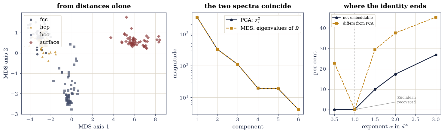
Fig. 83 Classical multidimensional scaling of the same dataset, computed from the matrix of pairwise distances with the coordinates discarded. Left: the embedding, which reproduces the principal-component map of the previous figure to machine precision, up to the sign of each axis. Middle: the spectrum of the double-centred Gram matrix against the squared singular values from the singular value decomposition, which agree to fourteen digits — the numerical statement of the identity B = YYᵀ. Right: what happens when the Euclidean distance d is replaced by d^α. Any α other than 1 moves the embedding away from the principal-component one, but only α > 1 drives eigenvalues of B negative, the signature that no set of real points has those dissimilarities at all. Powers at or below 1 remain perfectly embeddable — they simply embed a different geometry.#
MDS eigenvalues vs PCA squared singular values: max relative difference 2.85e-15
MDS embedding vs PCA scores:                    relative difference     2.67e-15

powering the dissimilarity, d -> d**α:
  α = 0.5: differs from PCA by 2.28e-01, negative spectral weight -0.00 %  (still Euclidean)
  α = 1.0: differs from PCA by 2.53e-15, negative spectral weight  0.00 %  (still Euclidean)
  α = 1.5: differs from PCA by 2.94e-01, negative spectral weight  9.87 %  (NOT Euclidean)
  α = 2.0: differs from PCA by 3.75e-01, negative spectral weight 17.32 %  (NOT Euclidean)
  α = 3.0: differs from PCA by 4.53e-01, negative spectral weight 26.80 %  (NOT Euclidean)
Validation 3 — an identity, and its boundary#
Three checks. The MDS eigenvalues must match the squared singular values and the embedding must match the PCA scores, both to machine precision, which is Eq. 72 holding exactly for Euclidean input. And with a nonlinear dissimilarity the agreement must fail while the Gram matrix acquires appreciable negative eigenvalues — the signature that the dissimilarities are not distances between any real points at all, which is precisely when the two methods stop being the same method.
✓  the eigenvalues of the double-centred Gram matrix are the squared singular values of the data matrix, to machine precision: for Euclidean distances eq-mds-gram reconstructs Y Yᵀ exactly rather than approximately   [max relative difference 2.9e-15]
✓  so the embedding built from distances alone reproduces the principal-component projection, having never been shown a coordinate   [relative difference 2.7e-15]
✓  while every other exponent moves the embedding away from the principal-component one: the two methods coincide for the Euclidean distance specifically, and not for monotone rankings of dissimilarity in general   [α=0.5: 2.3e-01, α=1.5: 2.9e-01, α=2.0: 3.8e-01, α=3.0: 4.5e-01]
✓  and the two ways of failing are distinct. For α ≤ 1 the dissimilarities are still distances between real points — the spectrum stays non-negative and MDS returns a valid, merely different, embedding. Above α = 1 they stop being embeddable at all and a large share of the spectrum turns negative, which is Schoenberg's classical result showing up as an eigenvalue sign   [α=0.5: -0.0 %, α=1.0: 0.0 %, α=1.5: 9.9 %, α=2.0: 17.3 %, α=3.0: 26.8 %]
True
Exercise 4 — Choosing what to compute#
The practical problem behind all of this: a trajectory offers far more environments than can be computed at an expensive level of theory, and something must choose a few hundred. Random selection is the obvious baseline. Farthest-point sampling [IAGiofre+18] is the standard alternative, and comparing them honestly means being clear about what each optimises.
Part a) Implement farthest-point sampling and the coverage radius — the largest distance from any point in the dataset to its nearest selected point. Write this one yourself — the implementation is the lesson.
Part b) Compare the coverage achieved by farthest-point sampling against random subsets of the same size, across a range of sizes, using enough random draws that the comparison means something.
Part c) Ask what it costs. Report where the selected points come from, and decide whether a set chosen to cover the space is the set you would want to fit a model to.
k= 4: FPS coverage 3.421   random median 4.480   (1.31× worse)   FPS beats  86.2 % of 400 draws
k= 8: FPS coverage 2.268   random median 3.448   (1.52× worse)   FPS beats  99.5 % of 400 draws
k=16: FPS coverage 1.718   random median 2.747   (1.60× worse)   FPS beats 100.0 % of 400 draws
k=32: FPS coverage 1.225   random median 2.391   (1.95× worse)   FPS beats 100.0 % of 400 draws

of the 16 points FPS selects, 75 % come from the most disordered set, which is 20 % of the data
Fig. 84 Animation of farthest-point sampling on the principal-component map, one selection at a time. Each new point (amber, with the newest in red) is the one furthest from everything already chosen. The early picks go straight to the corners of the distribution, which is what makes the coverage fall so quickly, and is also why the selection is dominated by the most strongly displaced environments rather than by typical ones. The curve tracks the coverage radius against the random-selection baseline.#
Validation 4 — it wins at its own game, and that is the caveat#
Three checks. Farthest-point sampling must achieve a smaller coverage radius than the median random subset at every size, and must beat the overwhelming majority of individual draws once the subset is big enough to have a choice to make. And the selection must be visibly biased towards the extremes of the dataset — not a defect, but the direct consequence of the objective, and the reason coverage alone is the wrong criterion for assembling a training set.
✓  farthest-point sampling achieves a smaller coverage radius than the median random subset at every size tested, which is the guarantee it is built to provide   [k=4: 3.42 vs 4.48, k=8: 2.27 vs 3.45, k=16: 1.72 vs 2.75, k=32: 1.22 vs 2.39]
✓  and beats almost every individual random draw once the subset is large enough for the choice to matter, so the advantage is not an artefact of comparing against an unlucky baseline   [k=8: 99.5 %, k=16: 100.0 %, k=32: 100.0 %]
✓  while over-representing the most strongly displaced environments by more than a factor of two: a rule that seeks out whatever is furthest away will preferentially return outliers, which is what you want for coverage and not what you want for a training set meant to be accurate where the system actually spends its time   [75 % of picks from a set that is 20 % of the data]
True
Notebook summary#
We took the descriptors of §7.1 and asked the two questions that follow from having them: how to look at a dataset of environments, and how to choose a subset worth computing.
Building the ensemble came first, and mattered more than it looks. A perfect lattice gives every atom of a phase an identical environment, so a dataset of any size collapses to one point per phase; thermal displacement is what makes an ensemble continuous. Principal component analysis then produced a clean two-dimensional map carrying 96.5 % of the variance, on which the leading component sorts environments by coordination and disorder appears only in the third. It is a good picture, and it hides exactly the distinction §7.1 worked hardest for: fcc and hcp overlap, while bcc sits far away. What PCA maximises is variance, and nobody promised that variance and interest are the same direction.
Classical scaling, given only the pairwise distances and no coordinates at all, reproduced that map to fourteen digits — the identity \(\mathbf B = \mathbf Y\mathbf Y^\mathsf{T}\) holding exactly for Euclidean input. Powering the distance showed where that ends, and showed that it ends in two separate ways: any exponent other than one moves the embedding, but only exponents above one drive eigenvalues negative and so stop the dissimilarities being distances between real points at all. Below one they remain perfectly embeddable and simply embed a different geometry — which is the regime where scaling is doing something projection cannot.
Farthest-point sampling beat random selection on coverage radius at every subset size and in essentially every individual draw. It also took most of its picks from the most strongly displaced environments, which are a fifth of the data. That is not a bug in the algorithm; it is what minimising the worst-case gap means. A training set assembled this way is excellent at not being surprised and poor at being accurate where the system actually spends its time, which is why the practical recipe is usually a blend.
Outlook#
Nonlinear reduction. Sketch-map [CTP11] was designed for exactly this data, preserving distances in a chosen band rather than globally, on the argument that neither very near nor very far pairs carry the structure of interest. t-SNE and UMAP are the general-purpose relatives, with the standing caveat that distances in their output are not to be read quantitatively.
Choosing components as well as samples. The same greedy argument applied to columns rather than rows selects a subset of descriptor features, which is how one prunes a symmetry-function set from hundreds to dozens [IAGiofre+18].
Sampling with a purpose. Coverage is a proxy. Active learning selects instead the environments a model is currently most uncertain about, and retrains — usually a better use of an expensive calculation than covering a space uniformly. §7.3 fits the model this argument needs and measures what coverage-based selection actually buys, on an even pool and on an imbalanced one.
Beyond the linear map. The kernel trick applies to both methods here: kernel PCA and the SOAP kernel [BartokKCsanyi13] reduce in a feature space where the distinction between phases can be far more linearly separable than it is here.
References#
Albert P. Bartók, Risi Kondor, and Gábor Csányi. On representing chemical environments. Physical Review B, 87(18):184115, 2013. doi:10.1103/PhysRevB.87.184115.
Michele Ceriotti, Gareth A. Tribello, and Michele Parrinello. Simplifying the representation of complex free-energy landscapes using sketch-map. Proceedings of the National Academy of Sciences, 108(32):13023–13028, 2011. doi:10.1073/pnas.1108486108.
Giulio Imbalzano, Andrea Anelli, Daniele Giofré, Sinja Klees, Jörg Behler, and Michele Ceriotti. Automatic selection of atomic fingerprints and reference configurations for machine-learning potentials. The Journal of Chemical Physics, 148(24):241730, 2018. doi:10.1063/1.5024611.
Warren S. Torgerson. Multidimensional scaling: i. theory and method. Psychometrika, 17(4):401–419, 1952. doi:10.1007/BF02288916.