


6.3 Metadynamics: Nitric Acid on Graphene#
Notebook overview#
Ordinary molecular dynamics is trapped by barriers: a rare event like a bond breaking may never happen on a simulable timescale. Metadynamics breaks the trap. It picks a few collective variables (CVs), coordinates that describe the slow motion of interest, and periodically deposits a small repulsive Gaussian hill at the system’s current position in CV space. The growing bias fills up whatever basin the system sits in, eventually floating it over the barrier, and the sum of all the hills, inverted, is the free-energy surface.
This is the course’s exercise on metadynamics, applied to two nitric-acid molecules
over a graphene sheet, with the fast and cheap density-functional tight-binding
(DFTB) method for the forces. We take the course’s committed output: the trajectory of
the collective variables (the COLVAR log) and the list of deposited hills (the
HILLS log). We render the system, follow the collective variables — measuring
whether the bias actually drove them anywhere, which for this short run it did not —
and reconstruct the free-energy surface by summing the hills.
Provenance. This notebook develops Lecture 13 of the course (metadynamics, collective variables, and free-energy surfaces), an exercise designed by the author (Raymond Amador). The structure (
grly5x3_2hno3.xyz) and the metadynamics logs (COLVAR,HILLS) are the course’s own committed CP2K/DFTB results from a short “simple metadynamics” run. The full course credit is in the footer.
Reading a validation. Each task closes with a check against an independent fact: the composition of the system, whether the bias drove any exploration — measured on the biased part of the run, it stalled — and that the reconstructed surface is consistent with where the trajectory went. A ✗ flags a mismatch; a ✓ is strong evidence, not proof.
Scope. This is a deliberately short teaching run, so the free-energy surface is qualitative, the bias filling the explored basin rather than fully converging a barrier. Energies are the committed values (Hartree, to kcal/mol). For the method see Laio & Parrinello [LP02].
Theory in brief#
Collective variables#
A collective variable \(s(\mathbf R)\) is a function of the atomic coordinates chosen to capture the slow degree of freedom, here coordination numbers: a smooth count of how many atoms of one type lie within a cutoff of another (C–O between graphene and the acid, N–O within the acid, H–C for a hydrogen approaching the sheet). Coordination numbers vary continuously as bonds form and break, which makes them good reaction coordinates.
The metadynamics bias and the free-energy surface#
Every \(\tau\) steps a Gaussian of height \(W\) and width \(\sigma\) is added to the bias at the current CV value \(\mathbf s_t\):
The bias accumulates in the basins the system visits, raising their floor until the system spills into the next basin. In the long-time limit the bias becomes the inverse of the underlying free energy, so the free-energy surface is reconstructed by summing the deposited hills and flipping the sign, \(F(\mathbf s) \approx -V(\mathbf s)\).
Setup#
The Setup below holds this notebook’s data and instruments — nothing you are asked to build. It is collapsed so the building stays yours; expand it whenever you want the details.
Exercise 1 — The system#
The course placed two nitric-acid molecules above a sheet of graphene, 60 carbon atoms plus the two \(\mathrm{HNO_3}\), and ran DFTB molecular dynamics. We render the committed structure: the flat hexagonal carbon lattice with the small acid molecules hovering above it. Density-functional tight binding is what makes this affordable, an approximate, parametrised electronic structure that is orders of magnitude faster than full DFT, fast enough for the long biased trajectory metadynamics needs.
Part a) Render the graphene + nitric-acid system.
Part b) Confirm its composition (a carbon sheet plus two HNO₃).
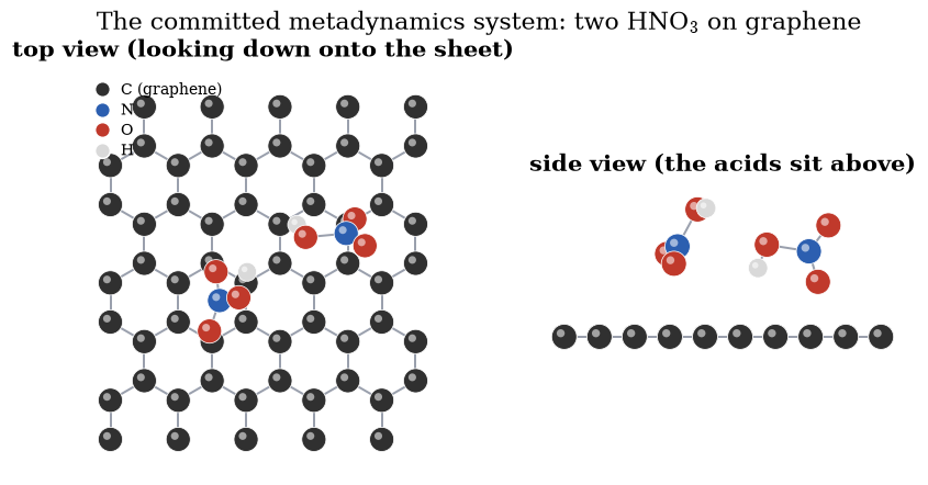
Fig. 71 The committed metadynamics system: a graphene sheet (60 carbon atoms, grey) with two nitric-acid molecules above it (nitrogen blue, oxygen red, hydrogen white). The forces come from density-functional tight binding, cheap enough for the long biased trajectory.#
composition: 60×C, 2×H, 2×N, 6×O
Validation 1 — graphene plus two nitric-acid molecules#
The system must be a carbon sheet (many C) with exactly the atoms of two HNO₃: two N, six O, two H.
✓ the system is graphene plus two nitric-acid molecules [composition {'C': 60, 'H': 2, 'N': 2, 'O': 6}]
True
Exercise 2 — The collective variables over time#
The COLVAR log records the three collective variables at every step. Plotting them
against time (Assignment 3) is the first look at what the run actually did, and the
question worth asking of the plot is not whether the variables move — they always do,
thermally — but whether the region they move in is still growing. Metadynamics that
is working pushes the system out of what it has already visited, so the explored range
keeps widening. Metadynamics that has stalled fluctuates about a fixed point, and the
range stops growing. The two look similar at a glance and are told apart by measuring.
Note
The first few logged samples are a startup transient, recorded before the first hill was deposited at \(t = 100\ \mathrm{fs}\), and they reach further in the C–O coordinate than the biased run ever does afterwards. Any statement about what the bias accomplished has to be made on \(t \ge 100\ \mathrm{fs}\); including the transient flatters the run with ground it covered before metadynamics had done anything.
Part a) Load COLVAR and plot the three CVs against time.
Part b) Decide whether the exploration is still expanding. Restricting to the biased part of the run, compare the range explored up to the end against the range already explored in the first quarter, and compare the drift of the quarter-by-quarter means against the size of the fluctuations about them.
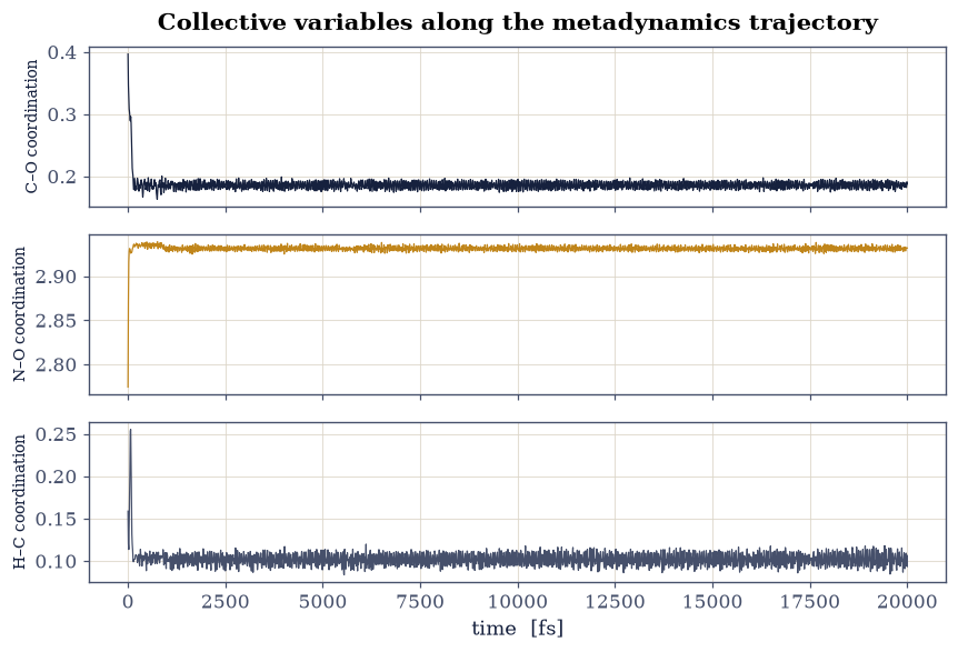
Fig. 72 The three collective variables (coordination numbers) along the metadynamics trajectory, from the committed COLVAR log. After a brief startup transient at the far left — recorded before the first hill was deposited — each variable settles and fluctuates about a fixed value for the remaining twenty picoseconds. The explored range stops growing almost immediately, which is the visual form of the diagnosis Exercise 4 makes quantitatively: the bias never pushed the system out of its initial basin.#
CV explored ranges: {'C–O coordination': np.float64(0.234), 'N–O coordination': np.float64(0.165), 'H–C coordination': np.float64(0.171)}
range growth (end / first quarter): {'C–O coordination': np.float64(1.0), 'N–O coordination': np.float64(1.0), 'H–C coordination': np.float64(1.06)}
quarter-mean drift / fluctuation: {'C–O coordination': np.float64(0.02), 'N–O coordination': np.float64(0.27), 'H–C coordination': np.float64(0.03)}
Validation 2 — the exploration has stalled#
The natural check here is the tempting one to get wrong. Asking merely that each collective variable cover a finite range passes on this data — but only on the strength of the pre-bias startup transient, so it would certify “the bias drove exploration” from samples recorded before a single hill existed. Measured on the biased run alone, the two statements below say the opposite and say it deterministically: the range explored by the end is the range that was already explored in the first quarter, and the mean of each variable drifts by a small fraction of its own fluctuation width. This is a stalled search, and recognising one is the skill.
✓ the biased run explores no more ground by the end than it had already covered in its first quarter: the search stopped expanding almost as soon as it started [range growth [1. 1. 1.06] (end / first quarter)]
✓ and each collective variable fluctuates about a fixed mean rather than migrating, the quarter-to-quarter drift being a fraction of the fluctuation it sits in [drift / fluctuation [0.02 0.27 0.03]]
True
Exercise 3 — Reconstructing the free-energy surface#
The HILLS log lists every deposited Gaussian: its centre in CV space, its widths,
and its height. Summing them and flipping the sign reconstructs the free-energy surface
Eq. 62 (Assignment 4). We project onto two of the variables, the C–O and H–C
coordinations that describe the acid approaching and bonding to the sheet, and contour
the result. The minimum marks the most-visited configuration; because this is a short
run the surface maps the explored basin rather than a fully converged barrier.
Part a) Load HILLS and reconstruct the 2-D free-energy surface.
Part b) Confirm its minimum coincides with where the trajectory spent the most time.
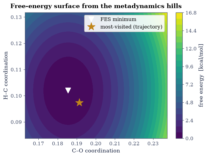
Fig. 73 Free-energy surface of the nitric-acid/graphene system, reconstructed by summing the metadynamics hills over the C–O and H–C coordination numbers (kcal/mol, relative to the minimum). The basin (dark) is the configuration the short run explored; the trajectory’s most-visited point (amber marker) sits in it, confirming the reconstruction. A longer run would extend the surface to neighbouring basins and the barriers between them.#
FES minimum at (0.19, 0.10); most-visited at (0.19, 0.10)
Validation 3 — the surface is consistent with the trajectory#
Metadynamics fills only the basins it visits, so the reconstructed free-energy
minimum must fall where the trajectory spent its time — a self-consistency check
that the HILLS reconstruction and the COLVAR trajectory tell the same story
(not an independent measurement: the hills are deposited along that trajectory).
✓ the reconstructed FES minimum sits where the trajectory spent the most time [FES min ↔ most-visited distance = 0.008 (3% of the explored span)]
True
Exercise 4 — Watching the hills fill, and asking whether they filled enough#
Exercise 3 summed all two hundred hills at once and read a free-energy surface off the total. That is the right final step, and it hides the two questions a metadynamics run has to answer before anyone may trust it: is the bias finished, and what flavour of metadynamics was this anyway.
Both are answerable from the committed HILLS file, and the first is easier to see
than to argue about — so accumulate the bias hill by hill and watch it. Each hill
is a Gaussian dropped at the system’s current position in collective-variable space,
so the bias grows fastest exactly where the system has spent the most time, which is
the bottom of a well. As a basin fills, the system stops returning to it and the
hills go elsewhere.
The diagnosis then follows from the shape of that growth. In standard metadynamics every hill has the same height, so the bias in a well-explored region keeps rising linearly for as long as the run continues — it never settles, and one has to stop and hope. Well-tempered metadynamics [BBP08] fixes this by shrinking each hill according to the bias already deposited where it lands,
so deposition slows as a region fills and the bias converges to a definite limit rather than growing without bound. The bias-growth curve tells the two apart at a glance: straight means standard and unconverged; bending over means well-tempered and settling.
Part a) Implement accumulate_bias(centres, widths, heights, GA, GB), returning
the bias on the grid after each hill — a running sum of Gaussians, one frame per
deposition. Project onto the same two collective variables Exercise 3 used, C–O and
H–C.
Write this one yourself — the implementation is the lesson.
Part b) Animate it, and diagnose the run. Check the recorded hill heights: are they constant? Then track the maximum bias against the number of hills deposited and compare its value after 20 hills with its value after 200. If the run were converging, the later hills would be adding less than the earlier ones.
Two further numbers in the same file are worth extracting, because together they say what the growth curve alone cannot. Compare the span of the hill centres in each collective variable against the hill width recorded beside them, and ask what a Gaussian several times wider than the whole explored region can possibly resolve. Then ask how much of the trajectory after the first hill lies inside the box the hill centres occupy. A run that is exploring should be leaving that box. Finally, measure how much the accumulated bias actually varies across that region, as a fraction of its own size — remembering that what pushes the system is the gradient of the bias and not its value, so a bias that rises uniformly is a bias that pushes on nothing.
Part c) Apply Eq. 63 to the same hill positions, with \(k_B\Delta T = 0.10\) in the units of the committed file, and re-accumulate. Compare the two growth curves and the height of the last hill against the first. This is the same trajectory rebiased under a different rule, so the difference is the rule and nothing else.
hill heights: constant to within 0.00e+00 -> standard metadynamics
standard bias max: 0.0598 (20 hills) -> 0.5993 (200 hills), ratio 10.02
well-tempered bias max: 0.0474 (20 hills) -> 0.1950 (200 hills), ratio 4.12
well-tempered last hill is 14.3 % of the first
hill width / explored span: 3.2x (C–O coordination), 4.5x (H–C coordination) -- the hills are wider than the search
97.9 % of the biased trajectory stays inside the box its own hills occupy
across that box the accumulated bias varies by only 4.4 % of its own height: an offset, not a gradient
Fig. 74 Animation of the metadynamics bias accumulating on the C–O / H–C collective-variable plane, hill by hill, from the course’s committed HILLS file. Left: the bias surface with the hill centres deposited so far marked in white. All two hundred centres fall in one small cluster, and the recorded hill width is several times wider than the region they cover, so every hill blankets the whole visible area at once: the panel brightens uniformly as the bias grows, varying by only a few percent of its height from corner to corner. Since the dynamics responds to the gradient of the bias rather than its value, a bias this flat pushes on nothing, which is why the cluster never spreads. Right: the maximum bias against the number of hills deposited, for the run as performed (navy) and for the same hill positions rebiased by the well-tempered rule of Eq. eq-well-tempered (amber). The navy curve is a straight line – the hallmark of standard metadynamics, whose fixed-height hills keep piling up indefinitely – while the well-tempered curve bends over as deposition slows in the filling basin.#
Validation 4 — a straight line is a warning, not a result#
Seven checks, all on the committed data and therefore deterministic. The recorded hill heights must be exactly constant, which identifies the run as standard rather than well-tempered. The bias must then grow linearly with hill count — tenfold more hills giving tenfold more bias — which is the quantitative statement that the run has not converged and that its free-energy surface is a lower bound on the exploration still to come. Applying the well-tempered rule to the same hills must bend that growth over, and its hill heights must decay. Two further checks pin the geometry of the search: the hills must be wider than the region their own centres cover, and the biased trajectory must still be sitting inside that region at the end, and the bias it accumulated must be nearly flat across it. Nothing here says the committed run is wrong; it says the run is short and its hills are coarse, both of which its own data is able to tell us.
✓ every recorded hill has the same height, so this is standard metadynamics and not the well-tempered variant of eq-well-tempered [got 0 vs expected 0 (rtol=1e-06, atol=1e-12)]
✓ and the bias grows LINEARLY with the number of hills: ten times the hills, ten times the bias, which is what a fixed-height rule must do in a region the trajectory keeps revisiting [got 10.0164 vs expected 10 (rtol=0.05, atol=1e-09)]
✓ the well-tempered rule applied to the same hill positions bends that growth over: deposition slows as the basin fills, which is what makes the bias converge to a limit instead of rising without bound [growth ratio 4.12 (well-tempered) vs 10.02 (as run)]
✓ and its hills shrink as they land in ground the bias already covers, while the total bias still rises monotonically [last well-tempered hill = 14.3 % of the first]
✓ the recorded hill width exceeds the span its own centres cover in BOTH collective variables, so no feature narrower than the whole explored region could have been resolved however long the run continued [width/span = 3.2 (C–O coordination), 4.5 (H–C coordination)]
✓ and the biased trajectory never escapes the box its own hills occupy: this run filled one basin without crossing out of it, which is the geometric statement of what the straight growth curve says arithmetically [97.9 % of the biased trajectory inside the hill box]
✓ and across that region the bias is nearly flat, varying by under a tenth of its own height: since the dynamics feels the GRADIENT of the bias, these hills raised the whole neighbourhood without pushing the system out of any part of it, which is the mechanism behind the two findings above [bias varies by 4.4 % of its height across the explored region]
True
Exercise 5 — Metadynamics run, not read#
Every exercise above reads a metadynamics log; nowhere in this course has anyone run metadynamics. This exercise closes that loop on a system where every answer is known in closed form: the double well \(V(x) = (x^2-1)^2\) — barrier exactly \(1\) at \(x=0\), minima at \(\pm1\) — under overdamped Langevin dynamics,
with the bias \(V_b\) grown by Gaussian deposition exactly as Eq. 62 prescribes. At \(k_BT = 0.12\) the barrier is \(8.3\,k_BT\): unbiased dynamics stays trapped for the whole observation window, and the deposition is what gets it out — the mechanism of the method, demonstrated rather than described. Afterwards the accumulated bias must be the free-energy surface it filled: \(V + V_b \approx\) const across the basin, checkable pointwise because \(V\) is analytic. The well-tempered variant shrinks its hills as Eq. 63 prescribes, and its bias converges to \(-\Delta T/(T+\Delta T)\,F\) — the rescaling that must be applied before its reconstruction is compared.
Part a) Implement the Langevin propagator with Gaussian deposition. Write this one yourself — the implementation is the lesson. Run unbiased and biased dynamics from the same start: the first must stay trapped over the window, the second must cross.
Part b) Test the reconstruction: \(V + V_b\) over the sampled region against a constant, with \(V\) known exactly.
Part c) Repeat with the well-tempered rule: the hills must decay, and the rescaled bias must reconstruct the same surface.
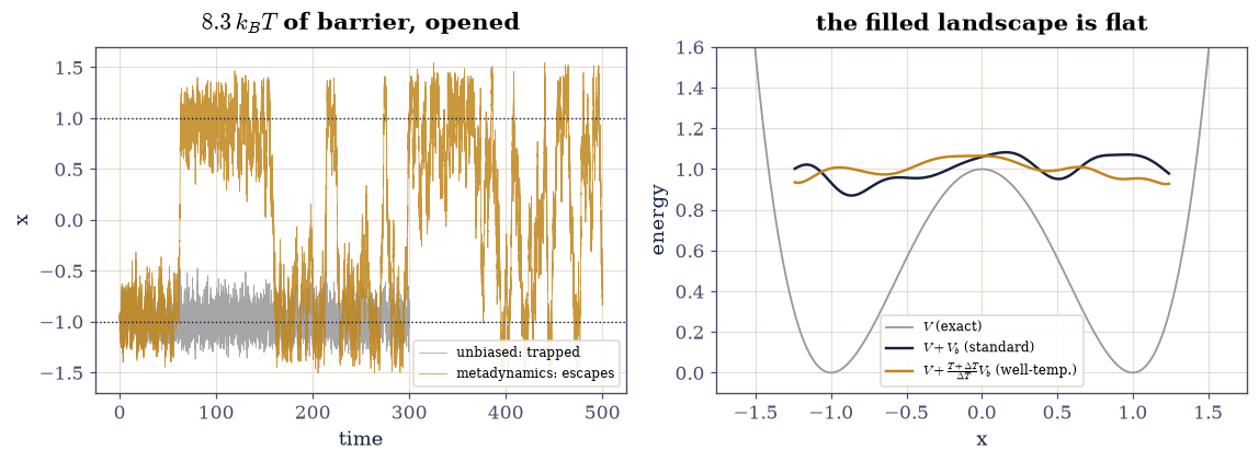
Fig. 75 Metadynamics run from scratch on the analytic double well under overdamped Langevin dynamics. Left: the trajectories — unbiased dynamics (grey) rattles in its starting well for the entire window at 8.3 kT of barrier, while the depositing run (amber) escapes within tens of time units and thereafter diffuses over both basins. Right: the filled landscape — the sum of the exact potential and the accumulated bias is flat across the sampled region to a few percent of the barrier (navy: standard deposition; amber: the well-tempered bias after its (T+ΔT)/ΔT rescaling), which is the method’s defining promise, checked against a closed form rather than against another simulation.#
unbiased: no crossing in 300 t.u.; metadynamics crosses at 62.5 t.u. (well-tempered: 213.8)
reconstruction flatness (std of V + bias over the basin): standard 0.0587, well-tempered (rescaled) 0.0399 (barrier = 1)
well-tempered hill decay: last hills at 22% of the first
Validation 5 — the method’s three promises, kept against a closed form#
Five checks. Unbiased dynamics must stay trapped over its whole window — the problem must exist before the cure is credited. The depositing run must cross, and fast. The filled landscape \(V + V_b\) must be flat across the basin to a few percent of the barrier, with \(V\) known exactly — the reconstruction promise, checked pointwise. The well-tempered hills must decay as Eq. 63 prescribes. And the well-tempered bias, after its \((T+\Delta T)/\Delta T\) rescaling, must reconstruct the same surface — the factor Exercise 4 could only state, here verified.
✓ unbiased Langevin dynamics stays trapped in its starting well for the entire window: at 8.3 kT of barrier there is a problem to solve [no crossing in 300 time units]
✓ the depositing run crosses within tens of time units: the growing bias is what opens the trap [first crossing at 62.5 time units]
✓ the filled landscape V + V_b is flat across the basin to a few percent of the barrier -- metadynamics' defining promise, checked against the closed-form V rather than against another simulation [std 0.0587 of a barrier of 1]
✓ the well-tempered hills decay as deposition proceeds, eq-well-tempered acting on a run this notebook performed rather than merely re-weighted [late hills at 22% of the first]
✓ and the well-tempered bias reconstructs the same surface once the (T+dT)/dT factor is applied -- the rescaling verified, not assumed [rescaled flatness 0.0399]
True
Notebook summary#
We followed a metadynamics run of nitric acid over graphene, computed with density-functional tight binding. The three coordination-number collective variables settle after a brief startup transient and then fluctuate about fixed values: measured on the biased part of the run alone, the ground explored by the end is the ground already explored in the first quarter. Summing the deposited Gaussian hills reconstructed the free-energy surface of the basin the system stayed in, and its minimum coincided with the trajectory’s most-visited configuration — a consistency check between the HILLS reconstruction and the independent COLVAR record, since the two come from different files.
Reading the HILLS file as a record of how the bias was built rather than only of what it summed to, we found the run diagnosing itself: constant hill heights identify it as standard rather than well-tempered metadynamics, the maximum bias grows strictly linearly with hill count, the trajectory never leaves the box its own hills occupy, and the hills are wider than that box in both collective variables — so wide that the accumulated bias varies by only a few percent across the region it covers. That last number is the mechanism behind the others: what drives the dynamics is the gradient of the bias, and hills too broad to build one raise the neighbourhood without pushing the system anywhere in it. Re-accumulating the same hill positions under the well-tempered rule bends the growth over and shrinks the last hill to a fraction of the first. None of that makes the committed calculation wrong — it makes it short, and short in ways its own output states plainly once the growth curve is plotted.
Outlook#
Convergence. A converged free-energy surface needs the bias to grow flat; the short run here does not reach that. Well-tempered metadynamics shrinks the hills over time and converges cleanly.
Choosing CVs. The result is only as good as the collective variables: a CV that misses the true slow mode leaves a hidden barrier. The exercise’s four candidate CVs (coordination numbers and a point-to-plane distance) are a study in that choice.
The dissociation. With a longer run the H–O bond of nitric acid breaks and the proton transfers, the dissociation the exercise is named for, appearing as a second basin across a barrier in the H–C coordination.
Reweighting. The deposited bias can be used to reweight the trajectory back to unbiased ensemble averages of other observables. Doing that honestly for the committed run would need the thermostat temperature in the same units as the HILLS energies, which the archive does not record — the double-well run of Exercise 5, where every unit is known, is the clean place the machinery lives.
References#
Alessandro Barducci, Giovanni Bussi, and Michele Parrinello. Well-tempered metadynamics: a smoothly converging and tunable free-energy method. Physical Review Letters, 100(2):020603, 2008. doi:10.1103/PhysRevLett.100.020603.
Alessandro Laio and Michele Parrinello. Escaping free-energy minima. Proceedings of the National Academy of Sciences, 99(20):12562–12566, 2002. doi:10.1073/pnas.202427399.