3.1 Molecular Dynamics of Lennard-Jones Clusters

Molecular and Materials Modelling

Volume III — Molecular Dynamics Notebook 3.1

Newton's equations in time: a velocity-Verlet integrator that conserves energy where Euler explodes, a thermostat that holds an argon cluster at 20 K, the radial distribution function that reads off its structure, and the melting that smears it away.

Based on FS 2023 · Lecture 9 (molecular dynamics)

Level · intermediate   •   Est. · 90–120 min

Raymond Amador v1.2.0  ·  2026-07-27  ·  CC BY 4.0 (text) / MIT (code)

Notebook overview

In Volume II we found the static structure of a Lennard-Jones cluster by sliding downhill to a minimum. Here we let it move. Integrating Newton’s equations in time turns the same potential into a trajectory: atoms vibrate about their lattice sites, the cluster holds its shape at low temperature and falls apart at high temperature, and the time-averaged structure becomes thermodynamics. This is the molecular-dynamics half of the cluster story, and the route to nearly everything measurable in a liquid or solid.

This is the exercise from Lecture 9, and we follow it. The course thermalized a 38-atom argon cluster in CP2K, in the canonical ensemble with a thermostat, then ran a microcanonical production simulation to extract the radial distribution function \(g(r)\). We show those input decks and reproduce the runs in Python, because CP2K’s classical engine here is again just the Lennard-Jones potential. We build the velocity-Verlet integrator, see why it conserves energy where a naive scheme does not, control temperature with a velocity-rescaling thermostat, compute \(g(r)\) from the trajectory, and watch the cluster melt.

Provenance. This notebook develops Lecture 9 of the course (molecular dynamics, ensembles, time integration, and the radial distribution function), an exercise designed by the author (Raymond Amador). The original ran CP2K (the thermalization_38.inp and production_38.inp decks shown in Exercise 1) on the Euler cluster; since the force field is exactly the Lennard-Jones potential, the dynamics are reproduced here in Python, and the analysis (\(g(r)\), energy conservation, temperature) mirrors the original. The full course credit is in the footer.

Reading a validation. Each exercise closes with a check against something independent: a conservation law, the equipartition theorem, the known nearest-neighbour spacing. A ✗ flags a mismatch to track down, not a verdict; a ✓ is strong evidence, not proof.

Units and scope. We use reduced Lennard-Jones units, energies in \(\varepsilon\), lengths in \(\sigma\), masses in \(m\), so \(\varepsilon=\sigma=m=1\) and \(k_B=1\); temperature is then \(T^\ast=k_BT/\varepsilon\). The deck’s argon values \(\varepsilon=119.8\,k_B\,\)K and \(\sigma=3.405\,\)Å set the scale, so its target of \(20\,\)K is \(T^\ast=20/119.8\approx0.167\). For methods see Allen & Tildesley [AT17] and Frenkel & Smit [FS02]; the founding study is Verlet [Ver67].

Theory in brief

Equations of motion

Each atom obeys Newton’s second law with the Lennard-Jones force,

(28)\[m\,\ddot{\mathbf r}_i = \mathbf F_i = -\nabla_i E, \qquad E = \sum_{i<j} 4\varepsilon\!\left[\left(\tfrac{\sigma}{r_{ij}}\right)^{12}-\left(\tfrac{\sigma}{r_{ij}}\right)^{6}\right].\]

In reduced units \(m=1\), so the acceleration is the force. Integrated forward in time from initial positions and velocities, Eq. 28 is a deterministic trajectory, and the energy \(E+\tfrac12\sum_i m\dot{\mathbf r}_i^2\) is conserved.

Time integration: velocity Verlet

We advance the trajectory with the velocity-Verlet algorithm, the workhorse of molecular dynamics:

(29)\[\mathbf r(t+\Delta t) = \mathbf r(t) + \mathbf v(t)\,\Delta t + \tfrac12\mathbf a(t)\,\Delta t^2, \qquad \mathbf v(t+\Delta t) = \mathbf v(t) + \tfrac12\big[\mathbf a(t)+\mathbf a(t+\Delta t)\big]\Delta t.\]

It is symplectic and time-reversible, which is why it conserves energy over long runs with no systematic drift, where a naive forward-Euler step (\(\mathbf r\!\to\!\mathbf r+\mathbf v\Delta t\), \(\mathbf v\!\to\!\mathbf v+\mathbf a\Delta t\)) pumps energy in and diverges. The price is a timestep \(\Delta t\) small enough to resolve the fastest vibration.

Ensembles and temperature

An isolated trajectory samples the microcanonical (\(NVE\)) ensemble: fixed particle number, volume, and energy. To fix temperature instead, the canonical (\(NVT\)) ensemble couples the system to a heat bath through a thermostat. The instantaneous temperature comes from the kinetic energy by equipartition, with \(3N-3\) degrees of freedom after removing the centre-of-mass motion,

(30)\[\tfrac12\textstyle\sum_i m\,\mathbf v_i^2 = \tfrac{1}{2}(3N-3)\,k_B T \;\;\Longrightarrow\;\; T = \frac{\sum_i m\,\mathbf v_i^2}{(3N-3)\,k_B}.\]

The simplest thermostat rescales every velocity by \(\sqrt{T_{\rm target}/T}\); the course used the gentler canonical velocity rescaling (CSVR) [BDP07], which adds the right fluctuations, but the rescaling idea is the same.

Structure: the radial distribution function

The radial distribution function \(g(r)\) is the probability of finding a pair of atoms a distance \(r\) apart, relative to an ideal gas of the same density:

(31)\[g(r) = \frac{1}{\rho\,N}\Big\langle \sum_{i\neq j}\delta(r-r_{ij})\Big\rangle \Big/ 4\pi r^2 .\]

Its peaks sit at the neighbour-shell distances, so a sharp first peak at the nearest-neighbour spacing \(r_{\min}=2^{1/6}\sigma\) signals a solid, and the smooth decay of a liquid signals lost long-range order. It is the simulation’s direct bridge to x-ray and neutron scattering.

---

Setup

The Setup below holds this notebook’s data and instruments — nothing you are asked to build. It is collapsed so the building stays yours; expand it whenever you want the details.

Show code cell source

Hide code cell source

import os

import numpy as np
import matplotlib.pyplot as plt
from scipy.spatial.distance import pdist, squareform

from ecp import validate

rng = np.random.default_rng(0)
# data: reduced-unit constants and the deck's physical targets. The force law and
# the velocity sampler are NOT here — they are this notebook's own machinery and are
# built in Exercise 1. What remains below is the cluster geometry, the .xyz reader
# that loads it, and two one-line observables.
RMIN = 2.0 ** (1.0 / 6.0)  # Lennard-Jones nearest-neighbour separation
SIGMA_AR, EPS_AR_K = 3.405, 119.8  # argon sigma [Å] and epsilon [K], from the deck
T_STAR_20K = 20.0 / EPS_AR_K  # reduced temperature of the deck's 20 K target
INK, AMBER, SOFT = "#16213e", "#c0851a", "#46506b"


def kinetic(v):
    """Total kinetic energy 1/2 Σ v^2 in reduced units (m = 1).

    Parameters
    ----------
    v : numpy.ndarray
        Velocities, shape (N, 3).

    Returns
    -------
    float
        The kinetic energy.
    """
    return 0.5 * np.sum(v * v)


def temperature(v):
    """Instantaneous temperature from equipartition (Eq. eq-temperature).

    Parameters
    ----------
    v : numpy.ndarray
        Velocities, shape (N, 3).

    Returns
    -------
    float
        The reduced temperature 2·KE / (3N - 3), centre-of-mass motion removed.
    """
    return 2.0 * kinetic(v) / (3 * len(v) - 3)


def data_file(name):
    """Locate a shipped data file, from the repo root (CI) or the notebook dir (Colab).

    Parameters
    ----------
    name : str
        File name under a ``data`` directory.

    Returns
    -------
    str
        The first existing path found.

    Raises
    ------
    FileNotFoundError
        If no candidate path exists.
    """
    for base in ("data", os.path.join("notebooks", "03-molecular-dynamics", "data")):
        path = os.path.join(base, name)
        if os.path.exists(path):
            return path
    raise FileNotFoundError(name)


def read_xyz(name):
    """Read a single-frame .xyz file.

    Parameters
    ----------
    name : str
        File name (coordinates in Å).

    Returns
    -------
    numpy.ndarray
        Coordinates of shape (N, 3) in the file's units (Å).
    """
    lines = open(data_file(name)).read().splitlines()
    n = int(lines[0].split()[0])
    return np.array([[float(v) for v in ln.split()[1:4]] for ln in lines[2 : 2 + n]])


# The course's relaxed 38-atom argon cluster, exactly as the MD decks read it in
# (data/38atoms.xyz, in Å). We convert to reduced units by dividing by σ and centre
# it; its Lennard-Jones energy is the LJ38 global minimum, −173.928 ε (Exercise 2.1).
cluster_A = read_xyz("38atoms.xyz")
cluster = (cluster_A - cluster_A.mean(0)) / SIGMA_AR
N = len(cluster)

Exercise 1 — Velocity Verlet and the microcanonical ensemble

This exercise is the engine of the original. The course thermalized the cluster with CP2K, whose thermalization_38.inp deck sets RUN_TYPE MD, ENSEMBLE NVT, TIMESTEP 0.5 fs, TEMPERATURE 20.0 K, and a CSVR thermostat, on the same METHOD Fist Lennard-Jones force field as before:

&MD
  ENSEMBLE NVT
  STEPS 10000
  TIMESTEP 0.5            ! femtoseconds
  TEMPERATURE 20.0        ! kelvin
  &THERMOSTAT
    TYPE CSVR             ! canonical sampling through velocity rescaling
  &END THERMOSTAT
&END MD

The decks ship with this notebook: thermalization_38.inp (canonical, with thermostat) and production_38.inp (microcanonical, ENSEMBLE NVE, no thermostat). We reproduce them by integrating Eq. 28 with velocity Verlet Eq. 29. With no thermostat the run is microcanonical, so the conserved quantity to watch is the total energy.

Part a) Implement lj_forces(x), returning the energy and the forces \(-\nabla E\) together. It is the same pair sum as §2.1 — broadcast displacements, numpy.fill_diagonal with inf to kill the self-terms, a factor \(1/2\) on the energy — but it returns the force, so mind the sign: the force is minus the gradient, and a sign slip here produces a beautifully stable trajectory of a cluster that flies apart. Write this one yourself — the implementation is the lesson.

Part b) Implement maxwell_velocities(T_star, seed_rng): draw each component from seed_rng.normal, subtract the mean so the cluster has no net drift, then rescale to hit \(T^\ast\) exactly using Eq. 30. Removing the drift matters — centre-of-mass motion is kinetic energy that never thermalises, so it would inflate every temperature you measure afterwards. Write this one yourself — the implementation is the lesson.

Part c) Implement run_md, one velocity-Verlet loop Eq. 29 with an optional velocity-rescaling thermostat. Verlet’s half-kick/drift/half-kick order is not a stylistic choice: it is what makes the map symplectic and the energy error bounded rather than growing. Write this one yourself — the implementation is the lesson.

Part d) Run the cluster in \(NVE\) from velocities drawn at \(T^\ast=0.1\) and confirm the total energy is conserved, and that the net momentum stays zero — the second is an independent check that the forces obey Newton’s third law.

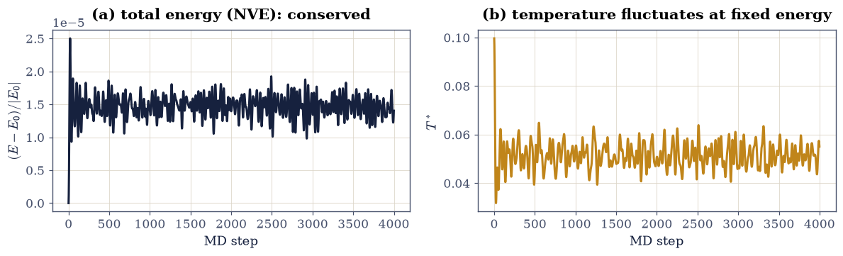
Fig. 26 A microcanonical (NVE) velocity-Verlet trajectory of the 38-atom argon cluster from velocities at \(T^\ast=0.1\): (a) the total energy stays flat (relative drift \(\sim10^{-5}\)), the hallmark of a correct symplectic integrator; (b) the temperature fluctuates freely, since at fixed energy only the sum of kinetic and potential energy is conserved.

Validation 1 — energy conservation in NVE

A correct microcanonical trajectory conserves the total energy: its relative drift over the run must be tiny, the molecular-dynamics equivalent of “did I integrate it right?”.

✓  velocity-Verlet NVE run conserves total energy   [max relative drift = 2.50255e-05 (limit 0.001)]
✓  the analytic forces are minus the gradient of the energy they are paired with: sign and normalisation both pinned   [max|Δ| = 4.90212e-08 (rtol=0.0001, atol=1e-05)]

True

Exercise 2 — Why velocity Verlet: the energy drift of Euler

The Verlet scheme is not the obvious one. The naive forward-Euler step, \(\mathbf r\to\mathbf r+\mathbf v\Delta t\) then \(\mathbf v\to\mathbf v+\mathbf a\Delta t\), looks just as reasonable but is not symplectic, and it pumps energy into the system until the trajectory is meaningless. Run both integrators from the same start and the difference is stark: Verlet’s energy stays flat, Euler’s climbs without bound. The drift also worsens with the timestep, which is why the course spent an assignment “converging the time steps”.

Part a) Integrate the same initial condition with Euler and with Verlet. Part b) Confirm Euler’s energy drift dwarfs Verlet’s.

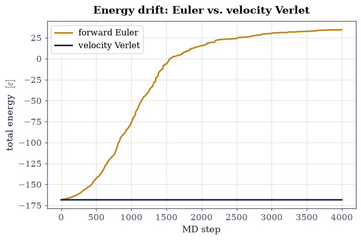
Fig. 27 Total energy along the same Lennard-Jones cluster trajectory, integrated with forward Euler (amber) and velocity Verlet (navy) at identical timestep \(\Delta t=0.004\). The symplectic Verlet scheme conserves energy; Euler pumps it in without bound, making the trajectory unphysical within a few thousand steps.

Validation 2 — Euler drifts, Verlet does not

At the same timestep the forward-Euler energy drift must exceed the Verlet drift by orders of magnitude, the quantitative reason molecular dynamics uses symplectic integrators.

✓  forward Euler drifts far more than velocity Verlet at equal timestep   [Euler drift = 1.2e+00, Verlet drift = 2.2e-05]

True

Exercise 3 — Temperature and thermalization (the canonical ensemble)

The microcanonical run holds energy fixed and lets temperature fluctuate. To prepare the cluster at a chosen temperature, as the course did before measuring anything, we couple it to a thermostat. The simplest version rescales every velocity by \(\sqrt{T_{\rm target}/T}\) at intervals, nudging the kinetic energy toward equipartition Eq. 30. Starting the cluster cold and thermostatting to the deck’s target \(T^\ast=20/119.8\approx0.167\), the temperature climbs and then settles, fluctuating about the target.

Part a) Thermalize the cluster to \(T^\ast=0.167\) with the velocity-rescaling thermostat.

Part b) Confirm the time-averaged temperature equals the target.

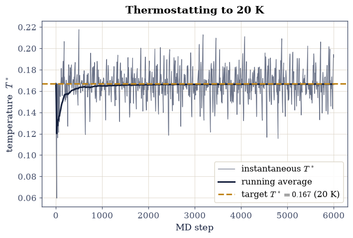
Fig. 28 Thermalization of the 38-atom argon cluster to the deck’s target \(T^\ast=20\,\mathrm{K}/119.8\,\mathrm{K}\approx0.167\) (amber line) with a velocity-rescaling thermostat. From a cold start the instantaneous temperature rises and settles, fluctuating about the target as the canonical ensemble requires; the running average (navy) converges to it.

Validation 3 — the thermostat reaches the target temperature

After equilibration the time-averaged temperature must equal the thermostat target \(T^\ast=0.167\), the defining property of a canonical simulation.

✓  thermostat holds the cluster at the target temperature   [got 0.166855 vs expected 0.166945 (rtol=0.15, atol=1e-09)]

True

Exercise 4 — The radial distribution function

With the cluster thermalized we measure its structure. The radial distribution function \(g(r)\) Eq. 31 is a histogram of pairwise distances, normalised by the \(4\pi r^2\) shell volume, accumulated over a microcanonical production trajectory (thermalize first, then run \(NVE\) and sample, exactly the canonical-then- microcanonical workflow of the two decks). For the cold solid cluster \(g(r)\) shows a sharp first peak at the nearest-neighbour spacing \(r_{\min}=2^{1/6}\sigma\) and further peaks at the next shells, the fingerprint of an ordered structure. Integrating that first peak (Assignment 8) gives the coordination number, the average count of nearest neighbours, well below the bulk fcc value of 12 for a cluster where most atoms sit on the surface.

Part a) Implement radial_distribution(frames).

Part b) Thermalize cold, run an \(NVE\) production trajectory, and locate the first peak of \(g(r)\). Part c) Read off the coordination number.

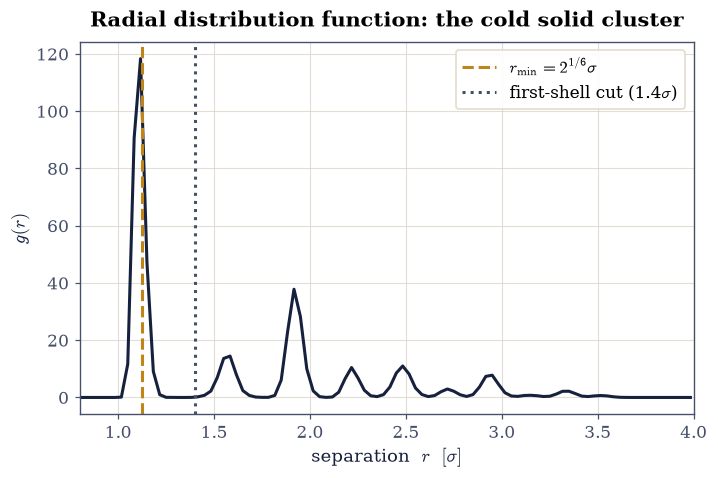
Fig. 29 Radial distribution function \(g(r)\) of the cold (solid) 38-atom Lennard-Jones cluster, from a microcanonical production trajectory at \(T^\ast\approx0.08\). The sharp first peak sits at the nearest-neighbour distance \(r_{\min}=2^{1/6}\sigma\) (amber line); the further peaks mark successive coordination shells, the structural signature of an ordered solid.

average coordination number = 7.6  (bulk fcc = 12; lower here, surface atoms)

Validation 4 — the first peak is the nearest-neighbour shell

The first peak of \(g(r)\) must sit at the Lennard-Jones nearest-neighbour distance \(r_{\min}=2^{1/6}\approx1.122\), where the pair potential is minimised.

✓  g(r) first peak sits at the nearest-neighbour distance   [got 1.11667 vs expected 1.12246 (rtol=0.06, atol=1e-09)]
✓  and the coordination number sits well below the bulk fcc value of 12, as it must for a 38-atom cluster whose atoms are mostly surface   [coordination = 7.6  (bulk fcc 12, isolated dimer 1)]

True

Exercise 5 — Melting the cluster

Raise the temperature and the cluster comes apart. Where the cold solid keeps atoms pinned near their lattice sites, giving a sharp \(g(r)\), a hot cluster has enough kinetic energy for atoms to diffuse past one another: the first peak broadens and the further shells wash out, the signature of a liquid (or, for a finite cluster, of melting and evaporation). The animation shows the hot cluster in motion, something no static structure can convey; we validate the physics of that motion, that its \(g(r)\) is measurably less ordered than the cold solid’s.

Part a) Run a cold and a hot production trajectory and compare their \(g(r)\). Part b) Animate the hot, melting cluster.

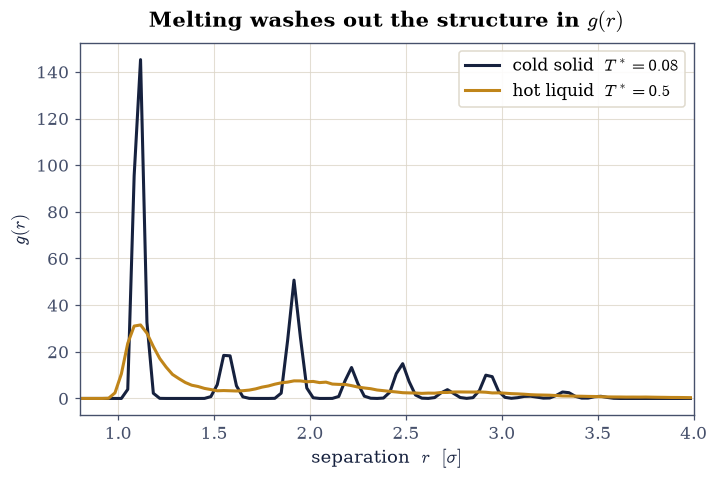
Fig. 30 Radial distribution functions of the 38-atom cluster, cold solid (\(T^\ast=0.08\), navy) versus hot liquid (\(T^\ast=0.5\), amber). Melting broadens the first (nearest-neighbour) peak and washes out the further coordination shells, leaving the smooth single-peak \(g(r)\) of a disordered liquid: the loss of long-range order made quantitative.

Once Loop Reflect

Fig. 31 Animation of the 38-atom argon cluster at \(T^\ast=0.5\), well above its melting point: atoms break from their lattice sites and diffuse over the surface and through the interior, the disordered motion whose time average gives the washed-out hot \(g(r)\). The amber atom is tracked to make the diffusion visible.

Validation 5 — the hot cluster is less ordered

Melting must register in \(g(r)\): the first peak of the hot trajectory is markedly lower (broader) than the cold solid’s, because diffusion has blurred the nearest-neighbour shell.

✓  the hot liquid g(r) is markedly less ordered than the cold solid   [first-peak height: cold 145.2 vs hot 31.5]

True

Exercise 6 — The spectrum of motion: the VACF, with the Hessian as referee

Everything measured so far is a static average. The velocity autocorrelation function

(32)\[c(t) \;=\; \frac{\langle \mathbf v(t_0)\!\cdot\!\mathbf v(t_0+t)\rangle} {\langle \mathbf v^2\rangle},\]

is where dynamics itself becomes an observable: its Fourier transform is the vibrational density of states, and its time integral is the Green–Kubo diffusion coefficient, \(D = \tfrac13\langle v^2\rangle \int_0^\infty c(t)\,dt\). One function, both faces of atomic motion — oscillation and transport.

The referee is exact. At low temperature the cluster is a harmonic solid, so the VACF’s spectrum must reproduce the normal-mode spectrum of the \(T=0\) minimum, which a finite-difference Hessian delivers independently: two entirely different computations, one on a trajectory, one on a single geometry, that are required to agree. And there is a trap with real teeth: a free cluster conserves angular momentum, so its velocity field carries a rigid-rotation component that never decorrelates. Left in, it floods the spectrum at zero frequency and drags every moment of it. The recorder must project out the same six modes — three translations, three rotations — that the Hessian analysis projects out of its matrix: one projector, in static and dynamic form.

Part a) Implement the velocity-recording MD loop and the rigid-motion stripper (instantaneous \(\boldsymbol\omega = \mathbf I^{-1}\mathbf L\) from the inertia tensor, then \(\mathbf v \to \mathbf v - \mathbf v_{\rm cm} - \boldsymbol\omega\times\mathbf r\)), the VACF via FFT, and a Welch-averaged spectrum. Write this one yourself — the implementation is the lesson.

Part b) Run cold (\(T^\ast = 0.02\)), and hold the spectrum against the Hessian’s 108 internal frequencies: centroid against mean frequency, and the fraction of spectral weight inside the Hessian’s band.

Part c) Melt it (\(T^\ast = 0.22\), above the §3.2 caloric-curve step) and read both faces: the spectrum grows a zero-frequency shoulder — the diffusive channel a solid does not have — and the Green–Kubo integral turns finite where the solid’s cancels. State the finite-cluster caveat honestly: atoms cannot diffuse forever in a bound droplet, so \(D\) here is an intermediate-time transport coefficient, read before the walls of the droplet are felt.

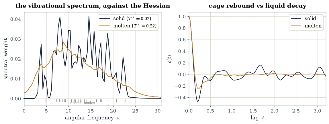
Fig. 32 Left: the vibrational spectrum of the 38-atom cluster from the Fourier-transformed velocity autocorrelation function, cold (navy) and molten (amber), with the 108 normal-mode frequencies of the T=0 minimum marked underneath (grey sticks). The cold spectrum lives almost entirely inside the Hessian’s band and its centroid agrees with the mean normal-mode frequency to under two percent — the harmonic approximation tested against dynamics, not assumed. The molten spectrum slumps toward zero frequency: the diffusive channel a solid does not possess. Right: the normalised VACF itself; the cold curve rebounds deeply negative as atoms bounce coherently in their cages, while the molten curve decays with only a shallow rebound, and its finite time integral is the Green–Kubo diffusivity.

VDOS centroid 12.89 vs Hessian mean 13.15 (2.0% apart); cold in-band weight 99.6%
low-frequency weight: solid 0.00%, molten 2.16%
Green-Kubo D: solid -0.00032, molten +0.00256

Validation 6 — dynamics agrees with statics, then departs from it

Five checks. The cold spectrum’s centroid must match the Hessian’s mean frequency and its weight must live inside the Hessian’s band — the harmonic approximation confirmed by an entirely independent computation. Melting must open the zero-frequency channel that the solid’s spectrum must not have. The Green–Kubo integral must be finite for the liquid and consistent with zero for the bound solid. And the solid’s VACF must rebound far below zero — the cage echo — where the liquid’s decays with only a shallow dip.

✓  the cold VACF spectrum's centroid agrees with the mean normal-mode frequency of the T=0 Hessian: a trajectory and a single-geometry diagonalisation, required to meet, and meeting   [got 12.8873 vs expected 13.1483 (rtol=0.1, atol=1e-09)]
✓  and essentially all cold spectral weight lies inside the Hessian's frequency band, so the solid's dynamics is its normal modes and nothing else   [in-band weight 99.6%]
✓  melting opens the zero-frequency channel: the molten spectrum carries low-frequency weight the solid's provably lacks -- the spectral face of diffusion   [low-frequency weight 0.00% -> 2.16%]
✓  the Green-Kubo integral is finite for the melt and consistent with zero for the bound solid -- transport appearing exactly where the spectrum said it would   [D_solid = -0.00032, D_molten = +0.00256]
✓  and the VACF itself tells the story in the time domain: the caged solid rebounds deeply negative, the liquid decays with only a shallow dip   [min c(t): solid -0.470, molten -0.251]

True

Notebook summary

We integrated the same Lennard-Jones cluster in time with velocity Verlet and confirmed it conserves total energy where forward Euler diverges, the practical reason molecular dynamics uses symplectic integrators. A velocity-rescaling thermostat held the real 38-atom cluster (the \(-173.93\,\varepsilon\) global minimum) at the deck’s \(20\,\)K, and the radial distribution function read off its structure: a sharp first peak at the nearest-neighbour distance \(r_{\min}=2^{1/6}\sigma\), an average coordination number near 8, and the washing-out of order on melting. Static structure, dynamics, and thermodynamics all came from one trajectory.

The deepening turned the trajectory itself into a spectrometer: the velocity autocorrelation function — recorded through the same six-mode projector the Hessian analysis uses, since a free cluster’s conserved angular momentum never decorrelates — reproduced the normal-mode spectrum of the \(T=0\) minimum to two percent, and on melting grew the zero-frequency shoulder and finite Green–Kubo integral that are diffusion’s spectral and temporal faces.

Outlook

• Real thermostats. The velocity rescaling here is crude; the course’s CSVR [BDP07], and Nosé-Hoover, sample the canonical ensemble correctly, with the right energy fluctuations rather than a hard rescale.

• The caloric curve. Average the potential energy over thermalized runs across a temperature grid; the kink where it rises steeply locates the cluster’s melting temperature, and the latent heat of the transition.

• Diffusion. The mean-squared displacement \(\langle|\mathbf r(t)-\mathbf r(0)|^2\rangle\) grows linearly in a liquid; its slope is the diffusion coefficient, zero in the solid and finite above melting.

• Bulk and periodic boundaries. The course also ran a bulk crystal with periodic boundaries (production_bulk.inp); with the minimum-image convention \(g(r)\) extends to many shells and yields the equation of state.

• Enhanced sampling. Replica exchange (Lecture 12) runs many temperatures at once and swaps between them, sampling melting and rare events far more efficiently than a single trajectory.

References

[AT17]

Michael P. Allen and Dominic J. Tildesley. Computer Simulation of Liquids. Oxford University Press, 2 edition, 2017.

[BDP07] (1,2)

Giovanni Bussi, Davide Donadio, and Michele Parrinello. Canonical sampling through velocity rescaling. The Journal of Chemical Physics, 126(1):014101, 2007. doi:10.1063/1.2408420.

[FS02]

Daan Frenkel and Berend Smit. Understanding Molecular Simulation: From Algorithms to Applications. Academic Press, 2 edition, 2002.

[Ver67]

Loup Verlet. Computer "experiments" on classical fluids. i. thermodynamical properties of lennard-jones molecules. Physical Review, 159(1):98–103, 1967. doi:10.1103/PhysRev.159.98.

Take this notebook with you

Use the download button (↓) in the toolbar above to save this notebook and run it yourself. The published notebooks ship without worked solutions; if you would like the reference solutions — to teach from or to check your own work — get in touch: hello@ramador.me.

Based on the lecture and exercise materials of Molecular and Materials Modelling (ETH Zürich and Empa, FS 2023), developed by Prof. Dr. Daniele Passerone (lectures), Dr. Carlo Pignedoli, and the author (exercises); here synthesised, expanded, and restyled by the author.