


2.1 Optimizing Lennard-Jones Clusters#
Notebook overview#
A handful of argon atoms, left to themselves, will settle into a compact little ball. Which ball is a surprisingly deep question. The atoms interact through the simplest realistic pair potential there is, yet the energy of an \(N\)-atom cluster, as a function of all \(3N\) coordinates, is a landscape of staggering complexity, with a number of local minima that grows roughly exponentially with \(N\). The 38-atom cluster is the textbook example: two competing funnels lead to two very different deep structures, and which one a geometry optimization finds depends entirely on where it starts.
This is the exercise from Lecture 3, and we follow it closely. The course ran the optimizations in CP2K on the Euler cluster; we show that very input deck and then reproduce it in Python, because CP2K’s classical engine here is the Lennard-Jones potential and nothing more. We relax the two 38-atom seeds the course used, a truncated octahedron and an icosahedron, and analyse each optimization the way the original did: energy, asphericity, and the Steinhardt order parameter \(Q_6\) as functions of optimization step. The payoff is the same one the course was built around. The truncated octahedron is the global minimum, a face-centred-cubic crystal fragment, and \(Q_6\) tells it apart from the icosahedron at a glance.
Provenance. This notebook develops Lecture 3 of the course (Lennard-Jones clusters, energy landscapes, geometry optimization, and order parameters), an exercise designed by the author (Raymond Amador). The original exercise drove CP2K’s classical force field (the
geo-opt.inpdeck shown in Exercise 2) on the Euler cluster; since that force field is exactly the Lennard-Jones potential, the optimization is reproduced here in Python so it is self-contained and checkable, while the analysis (asphericity and \(Q_6\) along the trajectory) mirrors the original. The full course credit is in the footer.
Reading a validation. Each exercise closes with a check against something independent: an analytic minimum, a tabulated global-minimum energy, a known order-parameter value. A ✗ flags a mismatch to track down, not a verdict; a ✓ is strong evidence, not proof.
Units and scope. We use reduced Lennard-Jones units, energies in \(\varepsilon\) and lengths in \(\sigma\), so \(\varepsilon=\sigma=1\). The original deck uses argon’s real values \(\varepsilon=119.8\,k_B\,\)K and \(\sigma=3.405\,\)Å, which is how the 38-atom coordinates (in Ångström) convert to reduced units below. For the landscapes picture see Wales, Energy Landscapes [Wal03]; for tabulated global minima, the Cambridge Cluster Database [WDD+].
Theory in brief#
The Lennard-Jones potential#
Two noble-gas atoms a distance \(r\) apart interact through the Lennard-Jones pair potential
The attractive \(-(\sigma/r)^6\) is the dispersion (induced-dipole) interaction that draws neutral atoms together; the repulsive \(+(\sigma/r)^{12}\) models the steep cost of overlapping closed electron shells, its exponent chosen as twice the attractive one for convenience. The well has depth \(\varepsilon\) at \(r_{\min}=2^{1/6}\sigma\), and \(\sigma\) is where \(V\) crosses zero. In reduced units the minimum sits at \(r_{\min}=2^{1/6}\approx1.122\) with \(V(r_{\min})=-1\).
Clusters and their energy landscape#
The energy of a cluster of \(N\) atoms is the sum over all pairs,
As a function of the \(3N\) coordinates this is a rugged surface with a vast number of local minima, each a mechanically stable shape, separated by barriers. Exactly one is the global minimum. A geometry optimization slides downhill from a starting structure to the nearest local minimum, here with the quasi-Newton L-BFGS method using the analytic forces \(-\nabla E\). For \(N=38\) the landscape has two deep funnels: a wide one ending at an incomplete Mackay icosahedron, and a narrow one holding the global minimum, a face-centred-cubic truncated octahedron just \(0.68\,\varepsilon\) lower. A downhill relaxation lands in whichever funnel its starting structure belongs to (Exercise 4’s disconnectivity graph makes the picture concrete).
Fingerprinting structure: asphericity and \(Q_6\)#
To recognise what structure an optimization found, two rotation-invariant numbers help. The asphericity, built from the principal moments of inertia \(I_1,I_2,I_3\),
is zero for a perfect sphere and grows as a cluster elongates. The Steinhardt order parameter [SNR83] averages spherical harmonics over the bonds and contracts over \(m\),
The \(l=6\) value cleanly separates structural families: a truncated-octahedron (fcc) cluster gives \(Q_6\approx0.57\), while the five-fold symmetry of an icosahedron makes its bond contributions largely cancel, leaving \(Q_6\approx0.13\).
Setup#
The Setup below holds this notebook’s data and instruments — nothing you are asked to build. It is collapsed so the building stays yours; expand it whenever you want the details.
Exercise 1 — The potential, the cluster energy, and the forces#
Everything rests on the energy Eq. 24 and its gradient; an optimizer converges far faster with exact forces than with finite differences. Differentiating, the force on atom \(i\) is \(-\nabla_i E=\sum_{j\neq i} 4\big(12\,r_{ij}^{-14}-6\,r_{ij}^{-8}\big)(\mathbf r_i-\mathbf r_j)\). The smallest clusters give a quick correctness check: three atoms relax to an equilateral triangle at \(E=-3\), four to a regular tetrahedron at \(E=-6\), every bond sitting at the well bottom.
Part a) Implement lj_energy_grad(x), returning the cluster energy
Eq. 24 and its flat gradient from a single call, so an optimizer can
use it for both fun and jac. Form every pair displacement at once by
broadcasting x[:, None, :] - x[None, :, :]; put numpy.inf on the diagonal of
the squared distances with numpy.fill_diagonal, which is what stops an atom
interacting with itself and turning the energy into nan; and halve the energy
sum, because the full matrix counts each pair from both ends.
Write this one yourself — the implementation is the lesson.
Part b) Wrap it as lj_energy(x), returning the energy alone for callers that
do not want the gradient.
Part c) Plot \(V(r)\) over \(r\in[0.9, 2.6]\), marking the minimum at \(r_{\min}=2^{1/6}\), \(V=-1\).
Part d) Confirm the dimer energy, check the analytic gradient against central finite differences, and verify that L-BFGS recovers the exact three- and four-atom minima, \(E=-3\) and \(E=-6\).
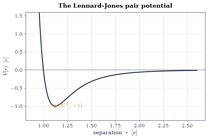
Fig. 19 The Lennard-Jones pair potential in reduced units (\(\varepsilon=\sigma=1\)): a steep short-range repulsion and a long-range \(-r^{-6}\) attraction give a well of depth \(\varepsilon\) at \(r=2^{1/6}\sigma\) (amber point), with \(V=0\) at \(r=\sigma\).#
Validation 1 — analytic forces and exact small-cluster minima#
The dimer at \(r_{\min}\) has energy \(-1\); the analytic gradient matches a central finite difference; and L-BFGS relaxes the 3- and 4-atom clusters to their exact global minima \(-3\) and \(-6\).
✓ LJ dimer minimum equals -1 [got -1 vs expected -1 (rtol=1e-09, atol=1e-09)]
✓ analytic LJ forces match finite difference [max|Δ| = 3.0246e-09 (rtol=0.0001, atol=1e-05)]
✓ L-BFGS recovers the exact LJ3 and LJ4 minima [max|Δ| = 1.95399e-14 (rtol=1e-05, atol=1e-09)]
True
Exercise 2 — The geometry optimization, as the course ran it#
This exercise is the heart of the original. The course optimized a 38-atom argon
cluster with CP2K, whose geo-opt.inp deck sets RUN_TYPE GEO_OPT with a
BFGS optimizer and, crucially, a METHOD Fist (classical) force field that is a
single Lennard-Jones term for argon:
&GEO_OPT
OPTIMIZER BFGS
MAX_ITER 500
&END GEO_OPT
...
&LENNARD-JONES
atoms Ar Ar
EPSILON 119.8 ! kelvin
SIGMA 3.405 ! angstrom
RCUT 8.4
&END LENNARD-JONES
The full deck ships with this notebook: geo-opt.inp.
So CP2K here computes exactly Eq. 24, and a faithful reproduction is
an L-BFGS relaxation of the same potential. We take the course’s
truncated-octahedron seed (38 argon atoms, in Ångström), convert it to reduced
units by dividing by \(\sigma=3.405\,\)Å, and relax it. It descends into the fcc
funnel and reaches the global minimum.
Part a) Relax the octahedral seed with local_minimize, which is the run the
original course performed with CP2K.
Part b) Show the initial and final structures side by side, and confirm the relaxed energy is the accepted global minimum \(-173.928\,\varepsilon\). Reaching it from this seed is not luck: the octahedral start already sits in the funnel that drains to it, which is exactly the point Exercises 4 and 5 complicate.
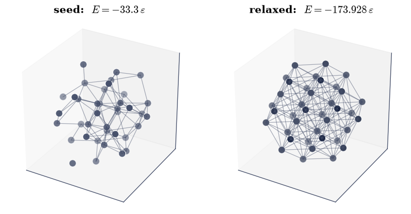
Fig. 20 The 38-atom octahedral seed before (left) and after (right) the Lennard-Jones geometry optimization. The crude initial guess relaxes into the compact, highly symmetric face-centred-cubic truncated octahedron, the global minimum at \(E=-173.928\,\varepsilon\).#
Validation 2 — the global minimum#
The octahedral seed must relax to the global minimum of the 38-atom cluster, the fcc truncated octahedron at \(E=-173.928\,\varepsilon\) (Cambridge Cluster Database).
✓ octahedral seed relaxes to the LJ38 global minimum [got -173.928 vs expected -173.928 (rtol=0.001, atol=1e-09)]
True
Exercise 3 — Tracking the optimization: energy, asphericity, \(Q_6\)#
The original exercise did not stop at the final energy; it watched the cluster
order as it relaxed, by computing observables along the optimization
trajectory. We do the same, on the course’s own committed optimization
trajectory (optimization-pos-1.xyz, 186 frames from a disordered seed to the
global minimum), shipped here downsampled as
lj38-optimization.xyz. The
asphericity Eq. 25 measures how
far from spherical the cluster is, and the Steinhardt \(Q_6\) Eq. 26
fingerprints the bond-orientational order. Plotted against optimization step, the
energy plunges, the asphericity stays small throughout (the cluster is compact from
the outset), and \(Q_6\) climbs to the fcc value \(\approx0.57\) as crystalline order
sets in.
Part a) Implement asphericity(x) from the gyration-tensor eigenvalues
Eq. 25, using numpy.linalg.eigvalsh on the \(3\times3\) tensor —
symmetric by construction, so the symmetric solver is both faster and free of
spurious imaginary parts.
Write this one yourself — the implementation is the lesson.
Part b) Implement a global steinhardt_q6(x) from Eq. 26,
averaging the bond spherical harmonics over every neighbour pair within the
cutoff before taking the modulus — averaging first is what makes \(Q_6\) a measure
of collective order rather than a sum of single-bond orientations.
Part c) Plot energy, asphericity and \(Q_6\) along the real CP2K trajectory, so the three fingerprints can be read against one another as the cluster orders.
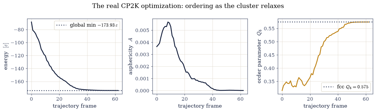
Fig. 21 Observables along the committed CP2K optimization from a disordered seed, versus step: the energy plunges to the global minimum, the asphericity stays small throughout (the cluster is compact from the outset), and the Steinhardt \(Q_6\) climbs to the fcc value 0.575 (dotted) as crystalline order sets in. This is the optimization watched from the inside.#
Validation 3 — the cluster orders into an fcc crystal#
Along the trajectory the energy must decrease, and the final structure must be nearly spherical (\(A\to0\)) with the fcc \(Q_6\approx0.575\), the quantitative signature of crystalline ordering.
✓ the real trajectory relaxes and rounds into a near-spherical crystal [E -68.4 → -173.9, asphericity 0.004 → 0.000]
✓ final Q6 equals the fcc value 0.575 [got 0.574371 vs expected 0.5745 (rtol=0.05, atol=1e-09)]
True
Exercise 4 — The other funnel: the icosahedron#
Now start from the course’s icosahedral seed. It relaxes into the other funnel, an incomplete Mackay icosahedron at \(E=-173.252\,\varepsilon\), just \(0.68\,\varepsilon\) above the global minimum yet structurally unrelated. Its five-fold symmetry is forbidden in any crystal, and the bond contributions to \(Q_6\) largely cancel, leaving \(Q_6\approx0.13\), far below the fcc value. So the two deepest structures of the 38-atom cluster sit in two separate funnels, and a downhill optimization is trapped in whichever it starts in. The disconnectivity graph, sketched below, is the standard picture of this [Wal03].
Part a) Relax the icosahedral seed and compare its energy, asphericity and \(Q_6\) with the octahedral minimum of Exercise 2. The two are close in energy and far apart in \(Q_6\), which is the whole reason a single order parameter is not enough to tell funnels apart.
Part b) Sketch the two-funnel disconnectivity graph, the standard picture of a landscape whose global minimum is not the one a quench usually finds.
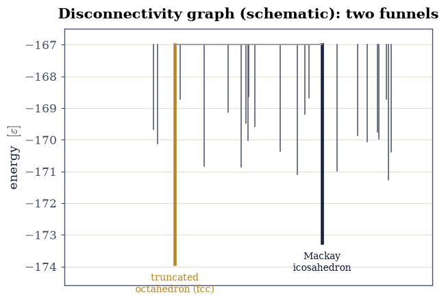
Fig. 22 Schematic disconnectivity graph of the 38-atom Lennard-Jones landscape: branches are local minima, drawn at their energies and joined at the energy of the lowest barrier between them. Two deep funnels dominate, the fcc truncated octahedron (global, amber, \(Q_6\approx0.57\)) and the Mackay icosahedron (navy, \(Q_6\approx0.13\)); a downhill optimization is trapped in whichever funnel its starting structure occupies.#
Validation 4 — two funnels, two fingerprints#
The icosahedral seed must relax to its funnel minimum \(-173.252\,\varepsilon\), which lies above the truncated-octahedron global minimum. And the order parameters must separate the two: the fcc truncated octahedron has the high \(Q_6\approx0.57\), the icosahedron the low \(Q_6\approx0.13\).
✓ icosahedral seed relaxes to its funnel minimum -173.252 [got -173.252 vs expected -173.252 (rtol=0.001, atol=1e-09)]
✓ the fcc truncated octahedron is the global minimum, and Q6 tells the two apart [E: octa -173.93 < icos -173.25; Q6: octa 0.57 vs icos 0.13]
True
Exercise 5 — When there is no good seed: global optimization#
The two seeds above were educated guesses, each already close to a funnel bottom. Without such a guess, finding the global minimum means searching the landscape, and the standard tool is basin-hopping [WD97]: perturb the current minimum, re-minimize, and accept the new minimum with a Metropolis criterion, walking the staircase of basins. We demonstrate it on the 13-atom cluster, small enough that basin-hopping reliably reaches its global minimum, a perfect icosahedron at \(E=-44.327\,\varepsilon\), from a random start. The 38-atom global minimum is far harder to reach this way, which is exactly what motivates the replica-exchange sampling of Lecture 12.
Part a) Run scipy.optimize.basinhopping on a random 13-atom cluster,
perturbing and re-minimising rather than descending once. A single L-BFGS run from
a random start lands in whichever basin it happens to begin in; basin-hopping
accepts or rejects minima, which is what lets it cross barriers a downhill
method cannot.
Part b) Animate the icosahedral global minimum and confirm its energy against the accepted LJ13 value.
Fig. 23 Animation of the 13-atom Lennard-Jones global minimum (\(E=-44.327\,\varepsilon\)), found by basin-hopping from a random start and rotated about the vertical: a central atom (amber) capped by twelve outer atoms forming a regular icosahedron, whose five-fold symmetry no crystal allows.#
Validation 5 — basin-hopping finds the LJ13 global minimum#
From a random start, basin-hopping must reach the tabulated 13-atom global minimum, \(E=-44.327\,\varepsilon\).
✓ basin-hopping reaches the LJ13 icosahedral global minimum [got -44.3268 vs expected -44.3268 (rtol=0.001, atol=1e-09)]
True
Exercise 6 — Finding a saddle by walking uphill along the softest mode#
Everything so far has gone downhill. But the objects that control kinetics — the transition states of §6.2 — are first-order saddle points: stationary points whose Hessian has exactly one negative eigenvalue. A saddle cannot be found by minimisation, and the standard single-ended answer is eigenvector-following: walk uphill along the softest Hessian eigenvector while relaxing in every direction perpendicular to it. The softest mode is the direction in which the basin’s restoring force gives way first; followed far enough, its curvature passes through zero and turns negative, and the walk converges onto the saddle at the top of the lowest escape path.
Two technical points carry the implementation. A free cluster has six zero Hessian modes (three translations, three rotations) that mean nothing and must be projected out before “softest” is well defined. And the Newton-like step \(s_i = -g_i/\lambda_i\) per eigenmode minimises along modes with \(\lambda_i > 0\) but maximises along the followed mode once its sign is handled — one algorithm, both behaviours, with a trust radius keeping every step honest where the quadratic model is not.
Part a) Catalogue the minima of LJ\(_7\) by local minimisation from random starts. Seven atoms have exactly four locally stable structures; their energies are known to the literature, and the lowest — the pentagonal bipyramid at \(-16.5054\,\epsilon\) — is the reference the saddle must sit above.
Part b) Implement the finite-difference Hessian, the zero-mode projector, and the eigenvector-following walk, and release it from the second-lowest minimum. Write this one yourself — the implementation is the lesson. Track the energy and the followed mode’s curvature along the walk: the curvature crossing zero is the moment the search leaves basin territory.
Part c) Certify the result the way Murrell–Laidler logic demands: the converged point must have exactly one negative internal Hessian eigenvalue, and steepest descent released along \(\pm\) that eigenvector must land in two different minima of the Part a catalogue — the two basins this saddle actually connects — with the saddle above both.
LJ7 minima found: ['-16.5054', '-15.9350', '-15.5932', '-15.5331', '-7.3196']
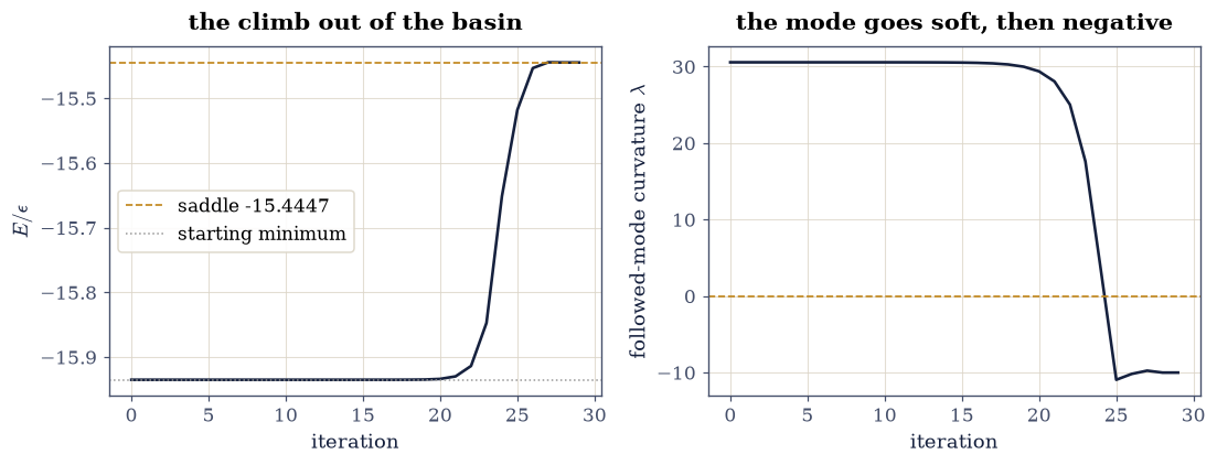
Fig. 24 Eigenvector-following on the LJ7 landscape, released from the second-lowest minimum. Left: the energy climbs monotonically out of the basin and flattens as the walk converges onto a stationary point. Right: the curvature of the followed mode — the softest internal Hessian eigenvalue — starts positive inside the basin, crosses zero where the walk leaves quadratic basin territory, and converges to a negative value: the signature of a first-order saddle. Steepest descent along the two directions of that negative mode lands in the global minimum and the starting minimum respectively, certifying which two basins the saddle connects.#
saddle: E = -15.4447, |g| = 4.2e-14, negative internal modes = 1
descent along -/+ the negative mode lands at [-16.5054, -15.935] (barriers 0.4903 and 1.0607)
Validation 6 — a certified transition state#
Four checks. The minima catalogue must contain the literature global minimum of LJ\(_7\), since everything is referenced to it. The walk must converge to a stationary point with exactly one negative internal eigenvalue — index one is the definition being verified, not a hope. The two descent paths must land in two distinct catalogued minima, which certifies the saddle’s connectivity, and the saddle must sit above both, as any saddle between them must.
✓ the catalogue contains the pentagonal-bipyramid global minimum of LJ7 at its literature energy [got -16.5054 vs expected -16.5054 (rtol=1e-06, atol=0.001)]
✓ the eigenvector-following walk converged to a stationary point of Hessian index exactly one -- the definition of a transition state, checked rather than assumed [|g| = 4.2e-14, negative internal modes = 1]
✓ steepest descent along the two directions of the negative mode lands in two DIFFERENT catalogued minima: the saddle's connectivity is certified, not presumed [descends to [-16.5054, -15.935]]
✓ and the saddle lies above both minima it connects, with the two barrier heights read directly off the energy differences [E_saddle = -15.4447 vs minima [-16.5054, -15.935]]
True
Exercise 7 — The double funnel weighed, and where its entropy actually lives#
Exercise 4 kept finding icosahedral structures instead of the fcc global minimum, and Exercise 5’s basin-hopping needed luck to cross between funnels. The thermodynamic question underneath: at temperature \(T\), which funnel should the cluster occupy? The harmonic superposition approximation [Wal03] answers it from quantities this notebook can compute exactly. Each minimum \(a\) contributes a classical partition function
with \(\omega_{a,i}\) its internal normal-mode frequencies and \(n_a\) its permutation–inversion degeneracy, \(n_a \propto 1/o_a\) for point-group order \(o_a\) — the truncated octahedron’s \(O_h\) has \(o = 48\), the icosahedral funnel bottom’s \(C_{5v}\) has \(o = 10\), so symmetry taxes the fcc structure by a factor \(48/10\) before any vibration is counted. Softer modes mean larger vibrational entropy; if the icosahedral minimum is soft enough, it wins above a crossover \(T^\ast\) despite its energy penalty.
Part a) Compute both minima’s internal frequency spectra from the projected finite-difference Hessians of Exercise 6, and establish which structure is vibrationally softer.
Part b) Assemble the two-state crossover temperature from Eq. 27 and confront it with two reference points: the cluster’s own melting temperature, \(T^\ast_{\rm melt} \approx 0.17\) from the replica-exchange data of §3.2, and the documented many-minima solid–solid crossover \(T^\ast_h \approx 0.12\) [DMW99]. The two-state answer is the finding: symmetry and softness together carry it to the right scale — but strand it just above melting, where a solid–solid transition cannot be observed. Quantify what closes the gap: the number of effective icosahedral minima needed to pull the crossover down to \(T^\ast_h\) turns out to be a mere handful.
Part c) Measure whether the landscape supplies that handful. Harvest the minima that local minimisation finds from random starts, classify each funnel membership by the global \(Q_6\) of Exercise 3, and count. The census delivers the missing minima many times over — and explains, in passing, why every downhill search of Exercise 4 kept landing icosahedral.
internal modes: 108 each; sum ln(omega_fcc/omega_ico) = 2.1385 (ico is softer)
two-state crossover T* = 0.182: the right scale, but above melting (0.17) and above the documented many-minima value (0.12)
closing the gap to T*_h = 0.12 takes ~7 effective low-lying icosahedral minima -- Part c asks whether the funnel has them
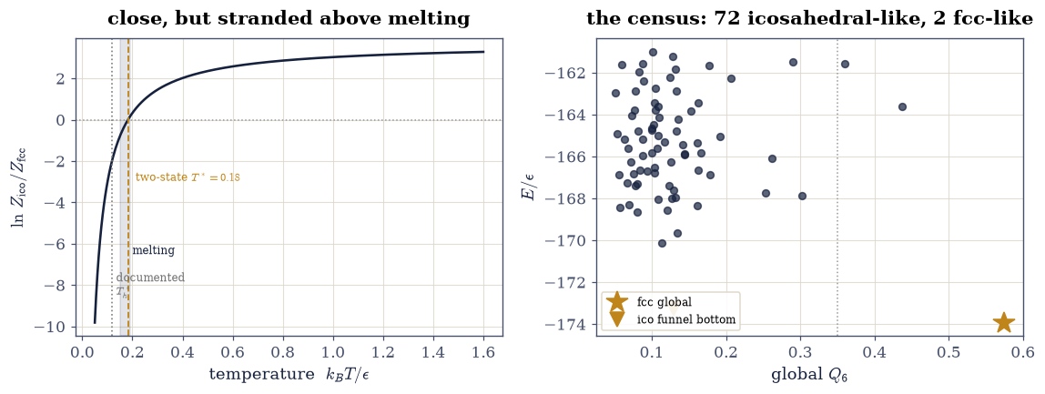
Fig. 25 Left: the two-state harmonic-superposition balance between the icosahedral and fcc funnel-bottom minima of LJ38, from Eq. eq-hsa with both 108-mode frequency spectra computed exactly. Symmetry (a 48/10 degeneracy penalty on the high-symmetry fcc structure) and vibrational softness together carry the crossing to the right scale — but strand it just above the melting band, where no solid–solid transition can be seen, and above the documented many-minima value near 0.12 (dotted). Closing that gap needs only a handful of additional low-lying icosahedral minima. Right: the census that supplies them many times over — minima harvested from eighty random starts, classified by the global Q6; nearly every basin found is icosahedral-like, the direct measurement of the configurational entropy the two-state model leaves out.#
census: 74 distinct minima from 80 starts; 72 icosahedral-like vs 2 fcc-like
Validation 7 — soft, symmetric, and nearly enough#
Four checks. Both spectra must be entirely positive (they are minima, and a negative mode would indict the relaxations, not the thermodynamics). The icosahedral minimum must be vibrationally softer — that is the entropic mechanism, and its sign is not negotiable. The two-state crossover must land at the right scale yet above both melting and the documented many-minima value, with the gap closed by a handful of effective extra minima — exactly computed, and honestly short. And the census must show the icosahedral funnel supplying that handful many times over.
✓ both funnel bottoms are true minima: all 108 internal modes positive in each spectrum, so the superposition inputs are sound [min omega: fcc 3.163, ico 4.144]
✓ the icosahedral minimum is vibrationally softer than the fcc global -- the sign of the entropic mechanism that must eventually favour it [sum ln(omega_fcc/omega_ico) = 2.139]
✓ the two-state crossover lands at the right scale yet above both melting and the documented many-minima value, and the factor that closes the gap is a handful of effective icosahedral minima -- configurational entropy finishing what symmetry and softness started [T*_two-state = 0.182 (melting 0.17, documented 0.12); n_eff ~ 7]
✓ and the census finds exactly that: random starts land in icosahedral-like basins overwhelmingly, the direct measurement of where the landscape's entropy lives -- and of why Exercise 4 kept finding the wrong funnel [74 minima: 72 ico-like vs 2 fcc-like]
True
Notebook summary#
We built the Lennard-Jones cluster energy from its pair potential and analytic forces, checked the forces against finite differences and small-cluster minima, and relaxed the course’s 38-atom seeds. The real CP2K optimisation trajectory carried the cluster from a disordered seed down to the global minimum at \(-173.93\, \varepsilon\), with the asphericity staying small throughout and the Steinhardt \(Q_6\) climbing to the fcc value \(0.575\). The icosahedral funnel landed at a distinct, higher minimum with \(Q_6\approx0.13\), and basin-hopping found the LJ13 global minimum unaided. These are three faces of one rugged landscape: local relaxation, structural fingerprinting, and global search.
The deepening then went where downhill methods cannot: eigenvector-following, built from a projected finite-difference Hessian, walked uphill out of the second LJ\(_7\) minimum and converged a certified index-one saddle — its two descent paths landing in exactly the two basins it connects. And the harmonic superposition weighed the LJ\(_{38}\) double funnel: symmetry and softness carry the icosahedral side to a crossover at the right scale but stranded just above melting, the missing factor being a handful of extra funnel minima that a census of eighty random relaxations supplies many times over.
Outlook#
Reaching the LJ38 global without a seed. Replica-exchange (parallel tempering) sampling, the subject of Lecture 12, crosses between funnels far more readily than basin-hopping and recovers the truncated octahedron from scratch.
Magic numbers. The Mackay icosahedra continue at \(N=55\) and \(147\); track \(Q_6\) and the asphericity as the structural families compete with growing \(N\).
The full disconnectivity graph. Enumerate minima and the transition states joining them to build the real graph rather than the schematic here; the 38-atom graph’s two branches are a landmark in the energy-landscapes literature [Wal03].
Real units. Argon’s \(\varepsilon=119.8\,k_B\,\)K and \(\sigma=3.405\,\)Å from the deck turn these reduced energies into physical binding energies and the structures into real noble-gas nanoclusters.
References#
Jonathan P. K. Doye, Mark A. Miller, and David J. Wales. The double-funnel energy landscape of the 38-atom lennard-jones cluster. The Journal of Chemical Physics, 110(14):6896–6906, 1999. doi:10.1063/1.478595.
Paul J. Steinhardt, David R. Nelson, and Marco Ronchetti. Bond-orientational order in liquids and glasses. Physical Review B, 28(2):784–805, 1983. doi:10.1103/PhysRevB.28.784.
David J. Wales. Energy Landscapes: Applications to Clusters, Biomolecules and Glasses. Cambridge University Press, 2003.
David J. Wales and Jonathan P. K. Doye. Global optimization by basin-hopping and the lowest energy structures of lennard-jones clusters containing up to 110 atoms. The Journal of Physical Chemistry A, 101(28):5111–5116, 1997. doi:10.1021/jp970984n.
David J. Wales, Jonathan P. K. Doye, A. Dullweber, and others. The Cambridge Cluster Database. https://www-wales.ch.cam.ac.uk/CCD.html. Tabulated global minima of Lennard-Jones and other clusters.