1.1 The Ising Model

Molecular and Materials Modelling

Volume I — Statistical Mechanics & Monte Carlo Notebook 1.1

The canonical lattice model of a magnet: the exact one-dimensional transfer-matrix solution, Landau's argument for why order needs two dimensions, a Metropolis Monte Carlo sampler checked against both the exact 1D thermodynamics and Onsager's exact 2D critical temperature, and the spin configurations that make the phase transition visible.

Based on FS 2023 · Lecture 2 (Monte Carlo)

Level · intermediate   •   Est. · 90–120 min

Raymond Amador v1.2.0  ·  2026-07-27  ·  CC BY 4.0 (text) / MIT (code)

Notebook overview

The Ising model is the hydrogen atom of statistical mechanics: a lattice of binary spins \(\sigma_i=\pm1\) that prefer to align with their neighbours. Despite its simplicity it is one of the very few interacting many-body systems that can be solved exactly (in one dimension by the transfer matrix, in two by Onsager’s celebrated 1944 calculation), which makes it the ideal place to learn Monte Carlo sampling: almost every number we measure can be checked against a known truth.

We treat the model from first principles. We write its Hamiltonian and energy, solve the one-dimensional chain exactly with the transfer matrix and use Landau’s domain-wall argument to see why it never orders at finite temperature, build the Metropolis algorithm and validate it against that exact 1D solution, and then cross into two dimensions, where a genuine phase transition appears at \(k_BT_c\approx2.269\,J\), and locate \(T_c\) from the Monte Carlo data and compare it to Onsager’s exact value.

Provenance. This notebook develops Lecture 2 of the course (the 2D Ising model and the foundations of Monte Carlo), whose exercise was developed by Dr. Carlo Pignedoli. It is here adopted, expanded (the exact 1D transfer-matrix solution and the finite-size-scaling analysis), reimplemented, and restyled by the author; the full course credit is in the footer.

Reading a validation. Each exercise ends with a check comparing a computed result to an independent fact: a ground-state energy, an exact limit, the transfer-matrix solution, Onsager’s \(T_c\). A ✗ does not by itself mean the physics is wrong: it means the output didn’t match what the check expected, which may be a real error, a different-but-valid convention, or simply Monte Carlo noise against too tight a tolerance. Treat a ✗ as a prompt to locate the discrepancy; a ✓ is strong evidence of correctness, not a proof.

Units and scope. We work in natural units \(J=1\), \(k_B=1\), so temperature is measured in units of \(J/k_B\). This is a working review, not a textbook chapter: for the statistical mechanics see Pathria & Beale [PB11], Goldenfeld [Gol92], and Newman & Barkema [NB99a]; for the exact results, Onsager [Ons44] and Yang [Yan52]; for the algorithm, Metropolis et al. [MRR+53].

Theory in brief

Magnetism and the Hamiltonian

At the atomic scale, magnetism arises from the spin of electrons (here idealised to two orientations \(\sigma=\pm1\)). In a ferromagnet a quantum-mechanical exchange interaction makes neighbouring spins prefer to align, producing a macroscopic magnetisation. The central question is: at what temperature does this order break down? Above it, thermal fluctuations win; below it, order survives.

Ernst Ising (1925) assigned a binary spin \(\sigma_i\in\{-1,+1\}\) to each lattice site \(i\) and wrote the total energy as a sum over nearest-neighbour pairs \(\langle i,j\rangle\) plus a coupling to an external field \(h\):

(1)\[\mathcal{H} = -J\!\sum_{\langle i,j\rangle}\sigma_i\sigma_j \;-\; h\sum_i \sigma_i .\]

With \(J>0\) the coupling is ferromagnetic: a parallel pair (\(\sigma_i\sigma_j=+1\)) lowers the energy by \(J\), so the system prefers order; the field \(h\) biases spins toward \(+1\). In one dimension with \(N\) spins and periodic boundary conditions (\(\sigma_{N+1}\equiv\sigma_1\)) this is \(\mathcal{H}_{1D}=-J\sum_i\sigma_i\sigma_{i+1}-h\sum_i\sigma_i\). Its ground state (\(T\to0\)) has all spins aligned at energy \(E_0=-NJ\). If \(d\) of the \(N\) bonds are antiparallel (a “domain wall” on each), the energy is \(E/J = -(N-d)+d = -N+2d\), so every domain wall costs \(2J\).

The exact one-dimensional solution: the transfer matrix

All thermodynamics follows from the partition function \(Z=\sum_{\{\sigma\}}e^{-\beta\mathcal{H}}\), with \(\beta=1/k_BT\). Naïvely this is a sum of \(2^N\) terms, but writing the Boltzmann weight as a product of bond factors turns it into a matrix product. Define the \(2\times2\) transfer matrix with \(K=\beta J\), \(h'=\beta h\),

(2)\[\begin{split}\mathbf{T} = \begin{pmatrix} e^{K+h'} & e^{-K} \\ e^{-K} & e^{K-h'} \end{pmatrix},\end{split}\]

so that with periodic boundaries \(Z=\operatorname{Tr}(\mathbf{T}^N)=\lambda_+^N+\lambda_-^N\), where the eigenvalues are

(3)\[\lambda_\pm = e^{K}\cosh(h') \pm \sqrt{e^{2K}\sinh^2(h') + e^{-2K}} .\]

In the thermodynamic limit \(N\to\infty\) only the larger eigenvalue survives, and the free energy per site is

(4)\[f = -k_BT\,\ln\lambda_+ .\]

Every observable is a derivative of this one scalar: magnetisation \(m=-\partial f/\partial h\), susceptibility \(\chi=\partial m/\partial h\), internal energy \(u=f-T\,\partial f/\partial T\), specific heat \(C=-T\,\partial^2 f/\partial T^2\). At \(h=0\) they take the closed forms

Quantity	Exact 1D result (\(h=0\))	Behaviour
Magnetisation	\(m=0\) for all \(T>0\)	no spontaneous order
Internal energy	\(u=-J\tanh K\)	smooth, bounded
Specific heat	\(C/k_B=K^2/\cosh^2 K\)	broad Schottky peak, no singularity
Susceptibility	\(\chi=\beta\,e^{2K}\)	diverges as \(T\to0\)

Why \(T_c=0\) in one dimension — Landau’s argument

The absence of order is not an accident of the algebra; it is a competition of energy and entropy. Introducing a single domain wall into an ordered chain costs energy \(\Delta E=2J\), but the wall can sit on any of \(N\) bonds, gaining entropy \(k_B\ln N\). The free-energy change is

(5)\[\Delta F = \underbrace{2J}_{\text{energy cost}} - \underbrace{k_BT\ln N}_{\text{entropy gain}} \xrightarrow{\,N\to\infty\,} -\infty \quad\text{for any } T>0 .\]

Domain walls are always favoured, so long-range order cannot survive at any finite temperature. What rescues order in two dimensions is geometry: there a domain wall is not a point but an extended loop of length \(\ell\), costing energy \(\propto J\ell\) while its entropy also grows only \(\propto \ell\). Below a finite temperature energy wins, and an ordered phase survives up to a genuine critical point.

Order in two dimensions: Onsager and Yang

Onsager solved the 2D square-lattice model exactly in 1944. From the self-duality condition \(\sinh(2K_c)=1\) the critical temperature is

(6)\[k_B T_c = \frac{2J}{\ln\!\big(1+\sqrt2\big)} \approx 2.269\,J ,\]

and Yang (1952) derived the spontaneous magnetisation below it,

(7)\[m(T) = \big(1 - \sinh^{-4}(2K)\big)^{1/8}, \quad T<T_c \quad (m=0 \text{ above}),\]

whose exponent \(1/8\) is the critical exponent \(\beta\) of the 2D Ising universality class (the susceptibility and correlation length carry \(\gamma=7/4\), \(\nu=1\)). On a finite lattice of side \(L\) the sharp transition is rounded into a peak shifted slightly above \(T_c\),

(8)\[T_{\rm peak}(L) = T_c + \frac{A}{L^{1/\nu}} = T_c + \frac{A}{L} \quad (\nu=1),\]

a finite-size effect we will see directly, and which, fit over several \(L\), is itself the standard route to the exact \(T_c\).

---

Setup

The Setup below holds this notebook’s data and instruments — nothing you are asked to build. It is collapsed so the building stays yours; expand it whenever you want the details.

Show code cell source

Hide code cell source

import numpy as np
import matplotlib.pyplot as plt
from scipy.optimize import brentq

from ecp import validate

# data: reproducibility is mandatory, so one seeded generator drives every draw.
rng = np.random.default_rng(0)

# data: natural units throughout — J = 1, k_B = 1, temperature in units of J/k_B.
J = 1.0

# data: Onsager's exact 2D critical temperature, Eq. (eq-onsager-tc). A closed-form
# constant of the model, not something this notebook derives — it is the yardstick
# every T_c estimate below is measured against.
Tc_onsager = 2.0 * J / np.log(1.0 + np.sqrt(2.0))

# data: series accents for emphasised curves.
INK, AMBER = "#16213e", "#c0851a"

Exercise 1 — The Hamiltonian and the energy of a configuration

A configuration of the 1D chain is an array of \(\pm1\). From Eq. 1 its energy sums \(-J\sigma_i\sigma_{i+1}\) over nearest-neighbour bonds (periodic boundaries, so site \(N-1\) couples back to site \(0\)), and the magnetisation per spin is the mean spin. The schematic below fixes the picture: the ringed spin couples only to its two neighbours, and those are exactly the bonds whose energy changes when it flips, the locality we exploit in the Metropolis step (Exercise 3).

Part a) Implement energy_1d(s) for a 1-D array of \(\pm1\), evaluating Eq. 1 as -J * np.sum(s * np.roll(s, -1)): rolling by one site pairs every spin with its right neighbour and wraps site \(N-1\) back onto site \(0\), so each bond enters exactly once. Pairing with both neighbours instead is the classic factor-of-two error, and Part c) is what catches it. Write this one yourself — the implementation is the lesson.

Part b) Implement magnetization(s) as the mean spin, s.mean(). Leave it shape-agnostic: the 2-D lattice of Exercise 5 reuses it unchanged.

Part c) Confirm that the fully aligned chain of \(N=64\) spins sits at the ground-state energy \(E_0 = -NJ\), with all \(N\) bonds satisfied.

Fig. 1 A periodic 1D Ising chain: each arrow is a spin \(\sigma_i=\pm1\) (up in navy, down in amber). The ringed spin couples only to its two nearest neighbours through the highlighted bonds; flipping it changes the energy over just those bonds, \(\Delta E = 2J\sigma_i(\sigma_{i-1}+\sigma_{i+1})\).

aligned N=64 chain: E = -64.0 (expect -64.0), m = +1.0 (expect +1.0)

Validation 1 — the ferromagnetic ground state

A chain with every spin aligned has all \(N\) bonds satisfied, so its energy must be exactly \(E_0=-NJ\). This pins the sign and normalisation of energy_1d.

✓  aligned 1D ground-state energy equals -NJ   [got -64 vs expected -64 (rtol=1e-12, atol=1e-09)]

True

Exercise 2 — Exact thermodynamics in 1D (the transfer matrix)

Implement the closed-form observables from the transfer-matrix solution (Eq. 2–Eq. 4) and plot them. The magnetisation is exact for any field; at \(h=0\) the energy, specific heat and susceptibility take the table forms above. Three features are worth seeing: the internal energy rises smoothly from \(-J\) (cold, ordered) to \(0\) (hot, random); the specific heat shows a broad Schottky peak with no singularity: the hallmark of no phase transition; and the susceptibility diverges only as \(T\to0\), the signature that order forms only at exactly zero temperature.

Part a) Implement exact_1d(T, J, h), returning the exact per-spin magnetisation, internal energy, specific heat and susceptibility of the 1-D chain from the transfer-matrix free energy Eq. 4, using the closed-form larger eigenvalue Eq. 3 rather than a numerical eigh — the closed form is exact and carries no eigenvector sign ambiguity. Write this one yourself — the implementation is the lesson.

Part b) Plot \(m\), \(u\), \(C\) and \(\chi\) against temperature on a shared figure (Fig. 2).

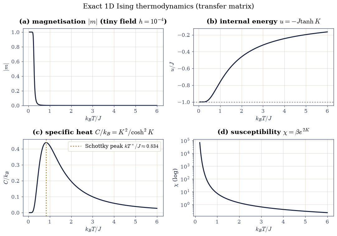
Fig. 2 Exact 1D Ising thermodynamics from the transfer matrix (Eq. eq-free-energy), with \(K=J/k_BT\): (a) magnetisation \(|m|\) under a tiny symmetry-breaking field \(h=10^{-4}\), which drives \(|m|\to1\) on the cold side (\(T\to0\)); at true zero field \(m=0\) for every \(T>0\); (b) internal energy per spin \(u=-J\tanh K\); (c) specific heat \(C/k_B=K^2/\cosh^2 K\) with its broad Schottky peak (amber); (d) susceptibility \(\chi=\beta e^{2K}\), diverging only as \(T\to0\). The absence of any singularity at finite \(T\) is the signature that the 1D model has no phase transition.

Validation 2 — exact limits and the Schottky peak

Three analytic facts pin the 1D solution: the internal energy tends to \(-J\) as \(T\to0\) (fully ordered) and to \(0\) as \(T\to\infty\) (fully random), and the specific-heat (Schottky) peak sits where \(K\tanh K=1\), i.e. \(k_BT^*/J\approx0.834\).

✓  1D internal energy → -J as T → 0   [got -1 vs expected -1 (rtol=1e-06, atol=1e-09)]
✓  1D internal energy → 0 as T → ∞   [got -0.001 vs expected 0 (rtol=1e-06, atol=0.001)]
✓  Schottky-peak temperature solves K tanh K = 1   [got 0.833557 vs expected 0.8336 (rtol=0.001, atol=1e-09)]

True

Exercise 3 — Metropolis Monte Carlo in 1D, checked against the exact solution

We cannot enumerate the \(2^N\) configurations, so we sample them with the Boltzmann weight \(P(\sigma)\propto e^{-\beta\mathcal{H}}\). The Metropolis recipe builds a Markov chain that does exactly this: propose flipping one spin, compute the energy change, and accept with probability \(\min(1,e^{-\beta\Delta E})\). Because only the bonds touching site \(i\) change, the energy change is local,

(9)\[\Delta E = 2J\,\sigma_i\sum_{j\,\in\,\mathrm{nn}(i)}\sigma_j ,\]

an \(O(1)\) quantity. This acceptance rule satisfies detailed balance with respect to the Boltzmann distribution, which is what guarantees the chain samples the correct ensemble. We update the chain a sublattice at a time (even sites, then odd): in 1D the even and odd sites are mutually non-adjacent, so all spins of one colour can be proposed at once, a vectorised Metropolis update that still respects detailed balance. The decisive test is that the sampled internal energy reproduces the exact transfer-matrix curve \(u(T)\).

Part a) Implement sweep_1d(s, beta, masks), one checkerboard Metropolis sweep of the chain in place: compute every local energy change at once with Eq. 1, accept with probability \(\min(1, e^{-\beta\Delta E})\) by comparing rng.random(s.shape) against np.exp(-beta * dE), and apply the even and odd sublattices in turn so that no two flipped spins are neighbours within one update. Write this one yourself — the implementation is the lesson.

Part b) Scan temperature and overlay the Monte Carlo internal energy on the exact \(u(T)\) of Exercise 2 (Fig. 3).

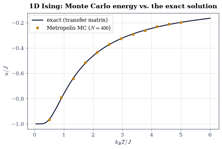
Fig. 3 Internal energy per spin of the 1D Ising chain: Metropolis Monte Carlo for \(N=400\) spins (amber points) against the exact transfer-matrix result \(u=-J\tanh(J/k_BT)\) (navy), confirming that the sampler reproduces the Boltzmann ensemble across the whole temperature range.

Validation 3 — Monte Carlo reproduces the exact 1D energy

The sampled internal energy must match the transfer-matrix curve across the whole temperature scan, an independent cross-method confirmation that the Metropolis chain samples the Boltzmann distribution.

✓  1D MC internal energy matches the exact transfer-matrix u(T)   [max|Δ| = 0.00791569 (rtol=0.03, atol=0.02)]

True

Exercise 4 — Space–time evolution and domain walls

Stacking successive snapshots of the chain (space across, Monte Carlo time down) makes the domain walls (the boundaries between \(+1\) and \(-1\) regions) visible as colour edges. At low temperature walls are rare and long-lived; at high temperature the chain is a fluctuating mess. This is the same physics as Eq. 5 seen dynamically: walls proliferate as \(T\) rises. We quantify it by counting walls (adjacent antiparallel pairs), which must increase with temperature.

Part a) Build a space–time history at low, intermediate and high \(T\). Part b) Count domain walls and check the count grows with temperature.

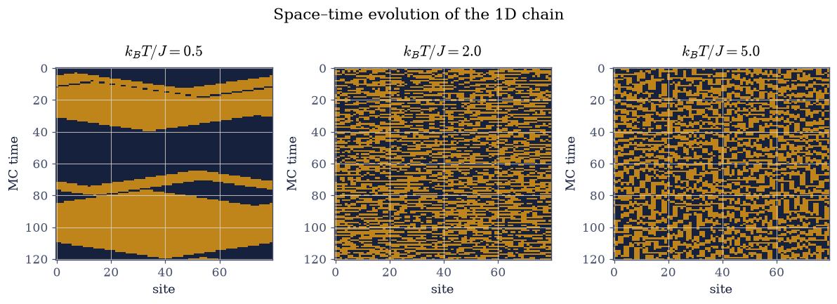
Fig. 4 Space–time histories of a periodic 1D Ising chain (horizontal = lattice site, vertical = Monte Carlo time; navy \(=+1\), amber \(=-1\)). At \(k_BT/J=0.5\) a few long-lived domains persist; at \(T=2.0\) walls appear and wander; at \(T=5.0\) the chain is fully disordered, the dynamical face of Landau’s argument, Eq. (eq-landau).

Validation 4 — domain walls proliferate with temperature

The equilibrium domain-wall count must rise monotonically from the cold chain to the hot one: the quantitative content of Landau’s energy–entropy competition.

✓  domain-wall count increases with temperature   [walls at T=[0.5, 2.0, 5.0]: [np.float64(1.2), np.float64(20.7), np.float64(33.0)]]

True

Exercise 5 — Into two dimensions: the order parameter vs. Onsager–Yang

In 2D a domain wall is an extended loop, so (as argued above) order can survive up to a finite \(T_c\). The Hamiltonian Eq. 1 and the Metropolis step Eq. 9 are unchanged; only the lattice topology differs, now with four neighbours. Scan temperature across Onsager’s \(T_c\approx2.269\) and compare the Monte Carlo magnetisation to Yang’s exact curve Eq. 7. As a second, parameter-free check we enumerate all \(2^{16}\) states of a \(4\times4\) lattice and confirm the sampler reproduces the exact Boltzmann \(\langle|m|\rangle\).

Part a) Implement nn_sum_2d, energy_2d and sweep_2d, the two-dimensional counterparts of Exercise 3. Build the neighbour sum by rolling the lattice along both axes with numpy.roll, and keep the checkerboard structure: on a square lattice the even and odd sublattices are exactly the two colours for which no site touches another of its own colour. Write this one yourself — the implementation is the lesson.

Part b) Plot the Monte Carlo \(\langle|m|\rangle\) against temperature together with the Onsager–Yang curve Eq. 7 (Fig. 5).

Part c) Cross-check the same quantity against the exact \(4\times4\) enumeration, which sums all \(2^{16}\) configurations directly and so owes nothing to the sampler.

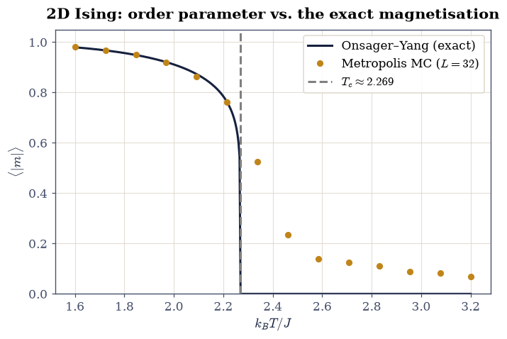
Fig. 5 Spontaneous magnetisation of the 2D Ising model: Metropolis Monte Carlo on an \(L=32\) lattice (amber points) against the Onsager–Yang exact \(m(T)=(1-\sinh^{-4}(2K))^{1/8}\) (navy, Eq. eq-yang), with Onsager’s \(T_c\) dashed. The order parameter falls from near \(1\) deep in the ordered phase to \(0\) above \(T_c\).

Validation 5 — exact 2D magnetisation, two ways

Deep in the ordered phase (\(T=2.0\)) the Monte Carlo magnetisation must match Yang’s exact value, and on the small \(4\times4\) lattice the sampler must reproduce the exact enumeration, a parameter-free check of the 2D sampler.

✓  2D MC |m| matches the Onsager–Yang exact magnetisation   [got 0.92001 vs expected 0.920816 (rtol=0.04, atol=1e-09)]
✓  2D MC ⟨|m|⟩ matches exact 4×4 enumeration   [got 0.722688 vs expected 0.729419 (rtol=0.06, atol=1e-09)]

True

Exercise 6 — Locating \(T_c\): the susceptibility and specific-heat peaks

The response functions measure fluctuations, which are largest where the system is poised between order and disorder. Through the fluctuation–dissipation relations

(10)\[\chi = \frac{N}{k_BT}\,\mathrm{Var}(m), \qquad \frac{C_v}{N k_B} = \frac{1}{N}\,\frac{\mathrm{Var}(E)}{(k_BT)^2},\]

both develop a peak at the transition. Use the signed magnetisation for \(\chi\): in a finite system \(|m|>0\) even in the disordered phase, so \(\mathrm{Var}(|m|)\) would understate the fluctuations. Two caveats shape what a finite run can tell us, and we return to them after the figure: on an \(L\times L\) lattice each peak sits slightly above \(T_c\) by \(O(1/L)\) (Eq. 8), and near \(T_c\) the dynamics slow critically, so \(\chi\), built from the slowly-decorrelating magnetisation, is noisier than \(C_v\) and its single-run peak less reliable. We therefore quote the specific-heat peak as our estimate of \(T_c\) and compare it with Onsager’s exact value Eq. 6; the result is Fig. 6.

Part a) Accumulate the susceptibility \(\chi\) and the specific heat \(C_v\) over a temperature scan, both from the fluctuation formulas Eq. 10 — variances of \(m\) and of \(E\) over the measured sweeps, not numerical derivatives of the mean, which would amplify the sampling noise.

Part b) Read \(T_c\) off the \(C_v\) peak with numpy.argmax and compare it to Onsager’s exact value. Mark the \(\chi\) peak as well, and note how much further it overshoots — the two estimators do not have to agree at finite \(L\), and the reason they do not is the subject of the next exercise.

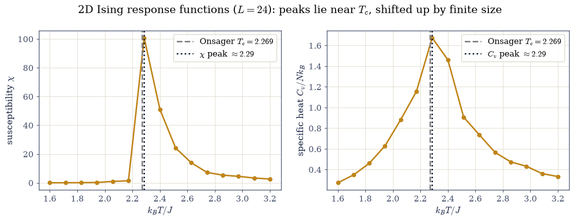
Fig. 6 Susceptibility \(\chi\) (left) and specific heat \(C_v/Nk_B\) (right) of the \(L=24\) 2D Ising lattice versus temperature (amber points), with Onsager’s exact \(T_c\) dashed and each measured peak dotted. Both peaks lie near \(T_c\) but above it, shifted by the finite-size relation Eq. (eq-fss) and scattered by critical slowing down; the susceptibility, built from the slowly-decorrelating magnetisation, is far noisier, so we read \(T_c\) off the steadier specific-heat peak.

Why the finite-size peaks overshoot \(T_c\)

On an infinite lattice both response functions diverge exactly at \(T_c\). On a finite lattice two distinct effects move the measured peaks upward, and together they make \(\chi\) the less reliable locator:

1. Finite-size shift. Rounding the divergence places each peak above \(T_c\) by \(T_{\rm peak}(L)-T_c\propto1/L\) (Eq. 8), with an observable-dependent amplitude. The shift shrinks with size: scanning \(L=16,24,32,48\) marches both peaks down toward \(2.269\).

2. Critical slowing down. Near \(T_c\) the autocorrelation time of single-spin Metropolis diverges as \(\tau\sim L^{z}\) (\(z\approx2.17\)). The susceptibility is built from fluctuations of the magnetisation (the slowest mode to decorrelate), so for a fixed sweep budget it is under-sampled exactly where it is largest, and its single-run peak scatters by a grid point or two: here it lands on the same grid node as the \(C_v\) peak, though run to run it drifts above or below. The energy decorrelates faster, so \(C_v\) is the steadier locator; raising the sweep count pulls the \(\chi\) peak back toward \(T_c\).

So neither peak is \(T_c\) on a finite lattice; both sit above it, and the \(C_v\) peak is the steadier of the two, which is why we quote it. The \(\chi\) peak’s larger run-to-run scatter is expected, not an error; the systematic route to the exact \(T_c\) is the finite-size-scaling extrapolation we carry out next, not any single lattice.

Validation 6 — finite-size \(T_c\) vs. Onsager

The headline result: the specific-heat peak of a stochastic simulation must land on Onsager’s exact \(T_c\), within a tolerance allowing for the finite-size upward shift Eq. 8 and the temperature-grid spacing.

✓  2D specific-heat peak locates Onsager's exact Tc   [got 2.28571 vs expected 2.26919 (rtol=0.06, atol=1e-09)]

True

Exercise 7 — Finite-size scaling: extrapolating to the exact \(T_c\)

The previous exercise left us with peaks that bracket \(T_c\) from above rather than pinpoint it. The cure is built into Eq. 8: because \(T_{\rm peak}(L)=T_c+A/L\) (with \(\nu=1\) for the 2D Ising model), the peak locations fall on a straight line when plotted against \(1/L\), and the line’s intercept at \(1/L\to0\) is \(T_c\) itself, the infinite-lattice limit, with the finite-size shift extrapolated away. We use the steadier specific-heat peak and read each one off its temperature scan with a parabolic fit to the three points around the maximum (a sub-grid estimate, since the true peak rarely lands exactly on a grid node).

Part a) For \(L = 12, 16, 24, 32\), scan a temperature window around \(T_c\) and locate the \(C_v\) peak of each with cv_peak_temperature.

Part b) Fit \(T_{\rm peak}\) against \(1/L\) with numpy.polyfit of degree 1, as Eq. 8 prescribes, and read \(T_c\) off the intercept (Fig. 7). The intercept is the \(L\to\infty\) limit, so it is the extrapolation — not any single lattice — that is compared with Onsager.

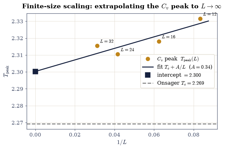
Fig. 7 Finite-size scaling of the 2D Ising specific-heat peak: the peak temperature \(T_{\rm peak}(L)\) for \(L=12,16,24,32\) (amber points) versus \(1/L\), with the linear fit \(T_{\rm peak}=T_c+A/L\) (Eq. eq-fss) extrapolated to \(1/L\to0\). The intercept (navy square) recovers Onsager’s exact \(T_c\) (dashed), free of the finite-size shift that displaces any single-lattice estimate.

Validation 7 — the \(L\to\infty\) intercept recovers Onsager’s \(T_c\)

Where any single finite lattice only brackets \(T_c\) from above, the extrapolated intercept must land on Onsager’s exact value, the payoff of finite-size scaling, turning the finite-size shift from a nuisance into a quantitative tool.

✓  finite-size-scaling intercept (L → ∞) recovers Onsager's exact Tc   [got 2.30027 vs expected 2.26919 (rtol=0.05, atol=1e-09)]

True

Exercise 8 — Equilibrium configurations and a low-temperature quench

Finally we look at the spins. Equilibrium snapshots show the phases directly: an ordered lattice far below \(T_c\), scale-invariant domains of every size at \(T_c\), and salt-and-pepper disorder above it. The dynamics are best seen moving: quench a random lattice to low temperature and animate it sweep by sweep: domains nucleate and coarsen, exactly the case where an animation shows what a still cannot. The quench can lock into a long-lived striped state (two domain walls wrapping the periodic lattice) whose magnetisation is small but whose energy is already deep, so we validate the robust quantity: the energy must fall far toward the ground state.

Part a) Show equilibrium configurations at three temperatures spanning the transition — well below, near, and well above \(T_c\) — as an imshow triptych (Fig. 8).

Part b) Animate a quench to \(T = 1.5 \ll T_c\) from a random start, and validate it on the energy of the final configuration rather than on the magnetisation: a lattice that orders into two stripe domains is genuinely low-energy while having \(m \approx 0\), so energy is the honest measure of ordering here and magnetisation is not.

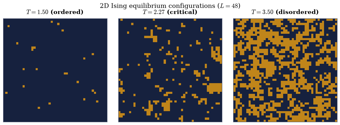
Fig. 8 Equilibrium 2D Ising configurations on a \(48\times48\) lattice (navy \(=+1\), amber \(=-1\)): ordered below \(T_c\), scale-invariant domains of all sizes at \(T_c\), and disorder above \(T_c\). At criticality the absence of a single domain size is the visual signature of the diverging correlation length.

Once Loop Reflect

Fig. 9 Animation of a low-temperature quench of a \(32\times32\) Ising lattice at \(T=1.5\ll T_c\): from a random start (navy/amber \(=\pm1\)), aligned domains nucleate and coarsen over Monte Carlo sweeps, driving the energy deep toward the ground state \(-2JN\).

Validation 8 — the quench orders the lattice (energetically)

A random start has energy per spin near zero; the ground state sits at \(-2J\) per spin. After 200 low-temperature sweeps the energy per spin must fall well below \(-1.5J\), robust evidence of ordering, whether into one domain or a low-energy stripe, independent of the final magnetisation.

✓  low-temperature quench drives the energy toward the ground state   [final E/N = -1.95 J  (ground state -2J),  |m| = 0.99]

True

Exercise 9 — How long is a Monte Carlo measurement worth? Autocorrelation

Every average so far has been quoted as if the \(n\) measured sweeps were \(n\) independent samples. They are not. A Metropolis sweep changes one spin at a time, so consecutive configurations look alike, and the number of statistically independent configurations is smaller — sometimes far smaller — than the number of sweeps. The quantity that measures this is the normalised autocorrelation function of an observable \(A\) at lag \(t\),

(11)\[\rho_A(t) = \frac{\langle A_k A_{k+t}\rangle - \langle A\rangle^2} {\langle A^2\rangle - \langle A\rangle^2},\]

and its sum, the integrated autocorrelation time

(12)\[\tau_{\rm int} = \tfrac12 + \sum_{t=1}^{\infty}\rho_A(t).\]

Its meaning is entirely practical: a run of \(n\) sweeps carries about \(n_{\rm eff} = n/2\tau_{\rm int}\) independent samples, so the error bar on \(\langle A\rangle\) is \(\sqrt{2\tau_{\rm int}}\) times larger than the naive \(\sigma/\sqrt{n}\) would suggest. Ignoring \(\tau_{\rm int}\) does not bias an average, but it makes the quoted uncertainty a fiction. The sum in Eq. 12 must be truncated in practice, because at large \(t\) the estimate of \(\rho_A\) is pure noise; the standard cure is Sokal’s self-consistent window, summing up to the first \(t\) with \(t \ge 6\tau_{\rm int}\) [NB99b, Sok97].

The reason this matters here is that \(\tau_{\rm int}\) is not a constant. As \(T\to T_c\) the correlation length diverges, and with it the time the algorithm needs to rearrange a correlated region: \(\tau_{\rm int}\sim L^{z}\) at \(T_c\), with a dynamic exponent \(z\approx 2.17\) for Metropolis in 2D. This is critical slowing down, and it is a property of the algorithm, not of the model — which is exactly what Exercise 10 exploits.

Part a) Implement integrated_tau(x) for a 1-D series: subtract the mean, form the autocorrelation with numpy.fft.rfft / numpy.fft.irfft on a zero-padded length \(2n\) (the padding is what makes the circular FFT correlation equal the linear one), normalise by lag-0 so \(\rho(0)=1\), then accumulate Eq. 12 and stop at the first \(t \ge 6\tau\). Write this one yourself — the implementation is the lesson.

Part b) Implement metropolis_series(L, T, n_eq, n_meas, seed), which equilibrates a random \(L\times L\) lattice for n_eq sweeps with the sweep_2d you built in Exercise 5 and then records \(|m|\) for n_meas further sweeps, driven by its own numpy.random.default_rng(seed).

Part c) Measure \(\tau_{\rm int}\) at \(T=T_c\) for \(L = 8, 12, 16, 24\) (300 equilibration and 3000 measurement sweeps each) and plot it against \(L\) on log axes. Confirm that \(\tau_{\rm int}\) grows with \(L\) — the growth is the slowing down. Read the effective exponent from a numpy.polyfit of \(\ln\tau\) against \(\ln L\), and treat it as indicative only: these runs are far too short, and the lattices far too small, to measure \(z\) properly.

tau_int at Tc: L=8: 2.6, L=12: 7.5, L=16: 17.0, L=24: 29.1
effective dynamic exponent z_eff = 2.24  (literature z ≈ 2.17)

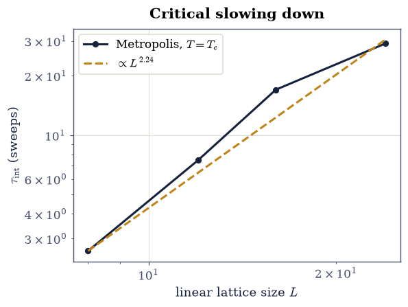
Fig. 10 Integrated autocorrelation time \(\tau_{\rm int}\) of \(|m|\) under Metropolis dynamics at \(T=T_c\), against linear lattice size \(L\) on logarithmic axes, from 3000 measurement sweeps per point. The dashed line is a power-law fit \(\tau_{\rm int}\propto L^{z_{\rm eff}}\); the growth is critical slowing down, and the fitted exponent is indicative only at these sizes and run lengths.

Validation 9 — the correlation time is real, and it grows

Two independent facts. An uncorrelated series has \(\tau_{\rm int}=1/2\) exactly, so feeding integrated_tau white noise must return that — this pins the normalisation and catches a factor-of-two error in Eq. 12. And the Metropolis correlation time must grow with \(L\) at \(T_c\): that growth is the slowing down, and it is checked as an ordering, not as a value, because \(z\) is not measurable at these sizes.

✓  an uncorrelated series has tau_int = 1/2, pinning the normalisation of eq-tau-int   [got 0.519772 vs expected 0.5 (rtol=0.25, atol=1e-09)]
✓  the Metropolis correlation time grows with L at Tc: critical slowing down   [tau_int = [2.6, 7.5, 17.0, 29.1] for L = [8, 12, 16, 24]]

True

Exercise 10 — Beating the slowdown: the Wolff cluster algorithm

Critical slowing down is the algorithm’s fault, so a different algorithm can escape it. The insight, due to Swendsen and Wang and sharpened to a single cluster by Wolff, is to stop flipping spins one at a time and instead flip a whole correlated region at once [NB99b, Wol89]. Pick a site at random; then grow a cluster outward, adding each aligned neighbour with probability

(13)\[p_{\rm add} = 1 - e^{-2\beta J},\]

and finally flip every spin in the cluster together. The move looks violent, yet it is accepted unconditionally: Eq. 13 is chosen so that the bias in building the cluster exactly cancels the Boltzmann cost of flipping it, which is what leaves the equilibrium distribution untouched. That cancellation is the whole design, and it is why \(p_{\rm add}\) cannot be any other function of \(\beta\).

Near \(T_c\) the clusters this recipe grows are themselves of order the correlation length, so one update rearranges a correlated region in a single step and the correlation time barely grows with \(L\) at all (\(z\approx 0.25\)). Far below \(T_c\) the same property becomes a liability: the cluster is essentially the whole lattice and every update merely flips the entire system, which is why cluster algorithms are a critical-region tool rather than a universal replacement.

Part a) Implement wolff_update(s, beta, r): choose a random site with r.integers(L), record its sign, then grow the cluster with an explicit stack (a Python list used with .pop()), adding a neighbour when it still carries the original sign and r.random() < p_add with \(p_{\rm add}\) from Eq. 13. Flip each spin as it joins — that is what prevents a site being added twice and removes any need for a separate visited-set. Wrap neighbour indices with % L for periodicity, and return the cluster size. Write this one yourself — the implementation is the lesson.

Part b) Implement wolff_series(L, T, n_eq, n_meas, seed), the cluster counterpart of metropolis_series from Exercise 9, returning both the \(|m|\) series and the mean cluster size.

Part c) At \(T=T_c\) on a \(32\times32\) lattice, measure \(\tau_{\rm int}\) for both algorithms (Metropolis: 400 equilibration and 4000 measurement sweeps; Wolff: 200 and 2000 cluster updates) and report the ratio. Plot the two \(|m|\) series over their first 400 steps so the difference is visible rather than merely tabulated.

Part d) On a \(16\times16\) lattice at \(T_c\), compare \(\langle|m|\rangle\) from the two algorithms. They sample the same distribution by different means, so agreement here is a genuine cross-method check of both implementations at once — a disagreement would indict sweep_2d, wolff_update, or both.

L=32: tau_metro = 33.9 sweeps, tau_wolff = 2.7 updates
        speed-up factor = 12.3
        mean cluster = 484 of 1024 spins
L=16:   <|m|> Metropolis 0.7155 vs Wolff 0.7090

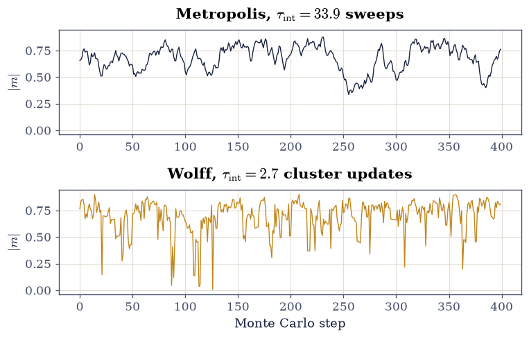
Fig. 11 Monte Carlo histories of \(|m|\) on a \(32\times32\) lattice at \(T=T_c\) under Metropolis sweeps (navy) and Wolff single-cluster updates (amber), over the first 400 steps of each. The Metropolis trace wanders slowly and stays near its previous value for many sweeps; the Wolff trace decorrelates within a few updates, because one cluster move rearranges a whole correlated region.

Validation 10 — same distribution, different dynamics

Three checks. The cluster the recipe grows at \(T_c\) must be a substantial fraction of the lattice, since that is the mechanism: flipping a correlated region in one move. The Wolff correlation time must be far below the Metropolis one at \(L=32\), which is the payoff. And the two algorithms must agree on \(\langle|m|\rangle\) at \(L=16\), where both are well converged — this is the check that matters most, because it is the only one that would fail if either update sampled the wrong distribution. All three are ratios or orderings rather than values, because \(\tau_{\rm int}\) from a finite chain is a noisy estimate.

✓  at Tc the Wolff cluster spans a sizeable fraction of the lattice, which is the mechanism that defeats critical slowing down   [mean cluster 484 of 1024 spins]
✓  and the cluster algorithm decorrelates far faster than Metropolis at Tc   [tau_metro/tau_wolff = 12.3]
✓  yet both algorithms sample the same equilibrium distribution: <|m|> agrees at L=16, a cross-method check of sweep_2d and wolff_update at once   [got 0.715451 vs expected 0.708986 (rtol=0.05, atol=1e-09)]

True

Exercise 11 — The Binder cumulant: a dimensionless number that knows \(T_c\)

Exercise 7 located the transition by extrapolating the drifting \(C_v\) peak, and needed a fit against \(1/L\) to do it. There is a sharper instrument. The Binder cumulant [Bin81] is a ratio of magnetisation moments,

(14)\[U_4(L, T) \;=\; 1 - \frac{\langle m^4\rangle}{3\,\langle m^2\rangle^2},\]

built so that the leading size dependences of numerator and denominator cancel. Its two off-critical limits are exact and worth deriving before running anything. Deep in the ordered phase \(P(m)\) is two sharp peaks at \(\pm m_0\), so \(\langle m^4\rangle = m_0^4 = \langle m^2\rangle^2\) and \(U_4 \to 2/3\). Deep in the disordered phase \(P(m)\) is a Gaussian of zero mean, for which Wick’s theorem gives \(\langle m^4\rangle = 3\langle m^2\rangle^2\) and \(U_4 \to 0\). Between the two, renormalisation-group scaling says \(U_4\) depends on \(L\) and \(T\) only through \(L^{1/\nu}(T - T_c)\) — so at \(T_c\) itself the \(L\)-dependence drops out entirely, and curves for different sizes cross there. No extrapolation, no fit: the crossing of two measured curves is the estimate. This is the standard production method for locating critical points, and Exercise 10’s cluster algorithm is what makes it affordable — every point below sits in the critical region, exactly where Metropolis is at its slowest.

Part a) Implement binder_u4(L, T_k, n_meas, seed): thermalise with Wolff updates, then accumulate \(\langle m^2\rangle\) and \(\langle m^4\rangle\) over n_meas further updates and return Eq. 14. Even powers only — under cluster updates \(m\) changes sign wholesale, so odd moments carry no information.

Part b) Sweep three lattice sizes across a temperature window bracketing \(T_c\) and plot the three curves with Onsager’s temperature marked. Check the two exact limits at the window’s ends.

Part c) Locate the pairwise crossings by interpolation, and compare the estimate against Exercise 7’s extrapolated \(C_v\) route: both should land near Onsager, but note what the cumulant did not need — a functional form for the finite-size drift.

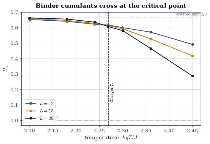
Fig. 12 The Binder cumulant of Eq. eq-binder for three lattice sizes across the critical region, computed entirely with Wolff cluster updates. Every curve starts at the exact two-peak limit 2/3 in the ordered phase and falls toward the exact Gaussian limit 0 in the disordered phase, but they do so in size-dependent fashion everywhere except at the critical point, where scaling makes the cumulant size-independent: the three curves cross within a percent of Onsager’s temperature (dashed). The crossing needs no extrapolation, which is its advantage over the drifting heat-capacity peak of Exercise 7.

U4(L=12) x U4(L=18): crossing at T = 2.2575 (Onsager 2.2692, off by 0.0116)
U4(L=18) x U4(L=28): crossing at T = 2.2564 (Onsager 2.2692, off by 0.0128)
U4(L=12) x U4(L=28): crossing at T = 2.2568 (Onsager 2.2692, off by 0.0123)
Exercise 7's extrapolated Cv route gave its estimate with a fitted 1/L form; the largest-pair crossing above needed no model at all.

Validation 11 — exact limits, one crossing each, and Onsager

Four checks. The largest lattice must sit at the exact two-delta limit \(2/3\) at the cold end of the window and fall well below it at the hot end, heading for the exact Gaussian limit — the two closed-form anchors of Eq. 14. Each pair of curves must cross exactly once in the window, which is the structural statement that the cumulant is size-independent at a single temperature. The ordering of the three curves must reverse across that temperature. And the largest pair’s crossing must land within three percent of Onsager’s exact \(T_c\) — with no extrapolation performed, which is the point of the exercise.

✓  at the cold end of the window the largest lattice sits at the exact ordered-phase limit 2/3, where P(m) is two sharp peaks   [got 0.662588 vs expected 0.666667 (rtol=1e-06, atol=0.03)]
✓  and at the hot end it has fallen far below 2/3, on its way to the exact Gaussian limit 0 of the disordered phase   [U4(L=28, T=2.45) = 0.287]
✓  each pair of curves crosses exactly once, and the size-ordering of the cumulants reverses across the crossing: size-independence happens at one temperature only, which is what makes U4 a locator of Tc   [sign changes [1, 1, 1]; ordering reverses between T=2.1 and T=2.45]
✓  and the largest-pair crossing lands within three percent of Onsager's exact critical temperature, with no extrapolation and no fitted functional form   [got 2.25638 vs expected 2.26919 (rtol=1e-06, atol=0.03)]

True

Notebook summary

We built the Ising model from its Hamiltonian and solved it two ways. In one dimension the transfer matrix gave the exact free energy and observables, which the Metropolis chain reproduced to within sampling error and which show no finite-temperature transition. In two dimensions the same sweeps recovered the Onsager–Yang spontaneous magnetisation, and the susceptibility and specific-heat peaks located the transition; extrapolating the steadier specific-heat peak to infinite size (finite-size scaling) recovered the exact critical temperature \(T_c = 2/\ln(1+\sqrt2) \approx 2.269\,J/k_B\). Along the way we met the concrete machinery of Monte Carlo: importance sampling, equilibration, fluctuation estimators, and the critical slowing-down that makes \(T_c\) hard to pin down — then beat it twice over: the Wolff cluster algorithm removed the slowdown, and the Binder cumulant it powers located \(T_c\) to a percent from the crossing of dimensionless curves, with no extrapolation and no fitted functional form.

Outlook

The Ising Hamiltonian is a template; changing the spin variable yields a whole family of models with qualitatively different physics:

Model	Spin \(\mathbf{s}_i\)	Key physics
Ising (\(q=2\))	\(\{\pm1\}\)	\(\mathbb{Z}_2\) symmetry, \(T_c>0\) in 2D
Potts (\(q\)-state)	\(\{1,\dots,q\}\)	first-order for \(q>4\) in 2D
XY	\(\theta_i\in[0,2\pi)\)	\(U(1)\); Berezinskii–Kosterlitz–Thouless transition
Heisenberg	\(\mathbf{s}\in S^2\)	\(O(3)\); realistic for many magnets
Random-field	Ising + disorder	order destroyed for \(d\le2\) (Imry–Ma)

The same structure also describes lattice gases (fluid transitions), binary alloys (phase separation), and Boltzmann machines (neural networks): the common thread being collective behaviour emerging from simple local rules.

Concrete extensions:

• Critical exponents. Near \(T_c\), \(\langle|m|\rangle\sim(T_c-T)^{1/8}\). Refine the grid below \(T_c\) and fit the exponent \(\beta=1/8\).

• Finite-size scaling, further. Exercise 7 fit \(T_{\rm peak}(L)=T_c+A/L\) at fixed \(\nu=1\); push to larger \(L\) (and more sweeps to tame critical slowing down), or let \(\nu\) float and fit \(T_{\rm peak}=T_c+A/L^{1/\nu}\) to measure the correlation-length exponent. The peak height of \(\chi\) scales as \(L^{\gamma/\nu}=L^{7/4}\), a second exponent from the same data.

• Cluster algorithms. Near \(T_c\) single-spin Metropolis suffers critical slowing down; the Wolff algorithm flips correlated domains at once and decorrelates far faster.

• The Binder cumulant \(U_4=1-\langle m^4\rangle/3\langle m^2\rangle^2\) crosses at \(T_c\) for all sizes, a sharper locator than the \(C_v\) peak [Bin81].

References

[Bin81] (1,2)

Kurt Binder. Finite size scaling analysis of ising model block distribution functions. Zeitschrift für Physik B, 43(2):119–140, 1981. doi:10.1007/BF01293604.

[Gol92]

Nigel Goldenfeld. Lectures on Phase Transitions and the Renormalization Group. Addison-Wesley, 1992.

[MRR+53]

Nicholas Metropolis, Arianna W. Rosenbluth, Marshall N. Rosenbluth, Augusta H. Teller, and Edward Teller. Equation of state calculations by fast computing machines. The Journal of Chemical Physics, 21(6):1087–1092, 1953. doi:10.1063/1.1699114.

[NB99a]

M. E. J. Newman and G. T. Barkema. Monte Carlo Methods in Statistical Physics. Oxford University Press, Oxford, 1999.

[NB99b] (1,2)

M. E. J. Newman and G. T. Barkema. Monte Carlo Methods in Statistical Physics. Oxford University Press, Oxford, 1999.

[Ons44]

Lars Onsager. Crystal statistics. i. a two-dimensional model with an order-disorder transition. Physical Review, 65(3–4):117–149, 1944. doi:10.1103/PhysRev.65.117.

[PB11]

R. K. Pathria and Paul D. Beale. Statistical Mechanics. Elsevier, 3 edition, 2011.

[Sok97]

Alan D. Sokal. Monte Carlo methods in statistical mechanics: foundations and new algorithms. In Cécile DeWitt-Morette, Pierre Cartier, and Antoine Folacci, editors, Functional Integration: Basics and Applications, volume 361 of NATO ASI Series B, pages 131–192. Springer, Boston, MA, 1997. doi:10.1007/978-1-4899-0319-8_6.

[Wol89]

Ulli Wolff. Collective Monte Carlo updating for spin systems. Physical Review Letters, 62(4):361–364, 1989. doi:10.1103/PhysRevLett.62.361.

[Yan52]

C. N. Yang. The spontaneous magnetization of a two-dimensional ising model. Physical Review, 85(5):808–816, 1952. doi:10.1103/PhysRev.85.808.

Take this notebook with you

Use the download button (↓) in the toolbar above to save this notebook and run it yourself. The published notebooks ship without worked solutions; if you would like the reference solutions — to teach from or to check your own work — get in touch: hello@ramador.me.

Based on the lecture and exercise materials of Molecular and Materials Modelling (ETH Zürich and Empa, FS 2023), developed by Prof. Dr. Daniele Passerone (lectures), Dr. Carlo Pignedoli, and the author (exercises); here synthesised, expanded, and restyled by the author.