


6.1 The Dehydration of Ethanol#
Notebook overview#
Heat ethanol over an acid catalyst and it loses water, leaving ethene: \(\mathrm{CH_3CH_2OH \to CH_2{=}CH_2 + H_2O}\). The reaction does not happen all at once; it passes through a transition state, a fleeting arrangement at the top of an energy barrier where the C–O bond is breaking and a C–H bond is migrating. The height of that barrier sets the rate, and computing it is a standard test of an electronic-structure method.
This is the course’s exercise on density functionals and basis sets, and its point is that the answer depends on the method. We take the course’s own optimised structures (reactant, transition state, products) and its committed total energies, computed with two functionals (PBE and B3LYP) across three basis sets (SZV, DZVP, TZVP), and build the reaction-energy profile, extract the activation barrier and reaction energy, watch them converge with basis-set size, and turn the barrier into a reaction rate.
Provenance. This notebook develops Lecture 7 of the course (the dehydration of ethanol, density functionals, and basis sets), an exercise designed by the author (Raymond Amador). The molecular structures (
ethanol.xyz,ethene.xyz,water.xyz,ts.xyz) and the total energies are the course’s own committed CP2K results; energies were computed with PBE and B3LYP. The full course credit is in the footer.
Reading a validation. Each task closes with a check against an independent fact: a transition state must lie above the reactant, the reaction is known to be endothermic, a converged barrier should match the measured one. A ✗ flags a mismatch; a ✓ is strong evidence, not proof.
Theory in brief#
Reaction profile and the barrier#
A reaction’s energy along its path rises from the reactant to a maximum at the transition state, then falls to the products. Two numbers summarise it: the activation barrier
which controls the rate, and the reaction energy \(\Delta E = E_{\rm products} - E_{\rm reactant}\), which says whether the reaction absorbs energy (endothermic, \(\Delta E>0\)) or releases it. Ethanol dehydration is endothermic and has a high barrier, which is why it needs heat and a catalyst.
Functionals and basis sets#
A density-functional calculation makes two approximations we can see here. The exchange-correlation functional (the generalised-gradient PBE, or the hybrid B3LYP that mixes in exact exchange) sets the underlying physics; the basis set (here the increasingly flexible SZV \(\to\) DZVP \(\to\) TZVP) sets how accurately the orbitals are represented. A result is trustworthy only once it has converged with basis-set size, and different functionals can still disagree after convergence: barriers are a sensitive probe of both.
From barrier to rate#
Transition-state theory turns the barrier into a rate constant through the Eyring (or, equivalently, Arrhenius) form
exponentially sensitive to the barrier, so the few-kcal/mol spread between methods becomes orders of magnitude in the predicted rate.
Setup#
The Setup below holds this notebook’s data and instruments — nothing you are asked to build. It is collapsed so the building stays yours; expand it whenever you want the details.
Exercise 1 — The reaction and its structures#
The course optimised four structures with CP2K: the ethanol reactant, the
transition state, and the ethene and water products. We render the
committed geometries. In the transition state the C–O bond has stretched and a
hydrogen is midway between carbon and the departing oxygen, the geometric signature of
a concerted dehydration. The CP2K input that produced them is a PBE deck; it ships
here: ethanol-pbe.inp.
Part a) Load and render the four structures.
Part b) Confirm the transition state’s stretched C–O bond.
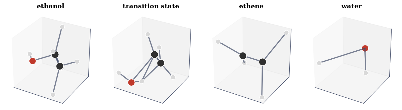
Fig. 60 The committed CP2K-optimised structures of the ethanol dehydration: the ethanol reactant, the transition state (the C–O bond stretched, a hydrogen migrating to the leaving oxygen), and the ethene + water products. Carbon grey, oxygen red, hydrogen white.#
shortest C–O distance: ethanol 1.43 Å -> transition state 1.90 Å (stretched)
Validation 1 — the transition state has a breaking C–O bond#
In the dehydration the C–O bond breaks, so the C–O distance must be markedly longer in the transition state than in the equilibrium ethanol (a normal C–O bond is ~1.4 Å).
✓ the transition state has a stretched (breaking) C–O bond [C–O: ethanol 1.43 Å → TS 1.90 Å]
True
Exercise 2 — The reaction-energy profile#
Now the energies. For each method the course computed the total energy of every species; the reaction profile is the energy relative to ethanol at three points along the path: reactant (zero by definition), transition state (the barrier), and products (ethene + water). We build it from the committed totals for all six method combinations (Assignment 5).
Part a) Assemble the profiles in kcal/mol.
Part b) Plot them and confirm every transition state lies above its reactant.
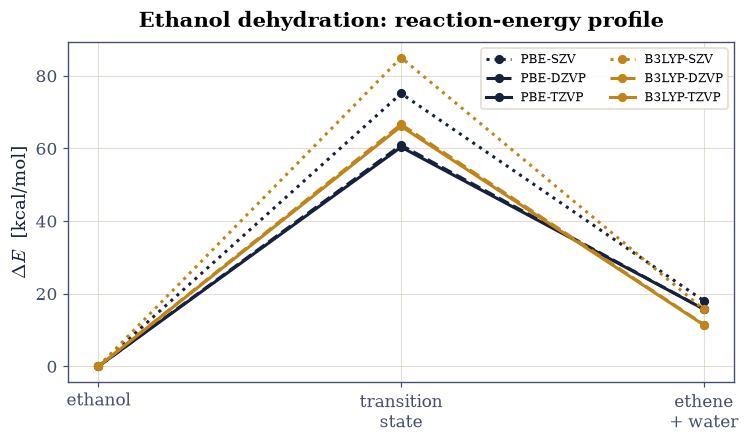
Fig. 61 Reaction-energy profiles for ethanol dehydration, from the course’s committed total energies: energy relative to ethanol (kcal/mol) at the reactant, transition state, and products, for PBE (navy) and B3LYP (amber) across three basis sets. Every path climbs a large barrier to the transition state and ends above the reactant (endothermic). The minimal SZV basis overshoots; DZVP and TZVP nearly coincide.#
Validation 2 — every transition state is a barrier#
A transition state is by definition a maximum along the path, so the barrier must be positive for every method, and the reaction must be endothermic (products above reactant) as ethanol dehydration is known to be.
✓ every method gives a positive barrier and an endothermic reaction [barriers 60–85, reaction energies 11–18 kcal/mol]
True
Exercise 3 — Convergence with functional and basis set#
The whole point of the exercise: how much do the method choices matter? Plotting the barrier against basis-set size for each functional shows the minimal SZV basis is far from converged, while DZVP and TZVP agree closely, so the basis is converged by triple-zeta. The two functionals still differ by a few kcal/mol at convergence, with the hybrid B3LYP-TZVP the most reliable estimate, landing near the experimental barrier of roughly 65–70 kcal/mol.
Part a) Tabulate barrier and reaction energy by method.
Part b) Confirm the basis is converged at TZVP and the B3LYP-TZVP barrier is in the experimental range.
method         barrier  reaction  (kcal/mol)
PBE-SZV           75.1      18.0
PBE-DZVP          60.9      15.8
PBE-TZVP          60.4      15.7
B3LYP-SZV         85.0      15.7
B3LYP-DZVP        66.6      11.5
B3LYP-TZVP        66.1      11.4
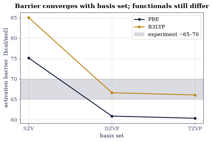
Fig. 62 Activation barrier of ethanol dehydration versus basis-set size for PBE (navy) and B3LYP (amber). The minimal single-zeta SZV basis overshoots badly; the barrier converges from DZVP to TZVP. At convergence the hybrid B3LYP-TZVP (~66 kcal/mol) sits in the experimental range (grey band, ~65–70 kcal/mol); PBE underestimates it.#
Validation 3 — converged at TZVP, and B3LYP lands on experiment#
The barrier must be converged by triple-zeta (DZVP and TZVP within a couple of kcal/mol), and the best method, B3LYP-TZVP, must fall in the measured range.
✓  the barrier is basis-set converged by TZVP (DZVP ≈ TZVP)   [|B3LYP DZVP − TZVP| = 0.53 kcal/mol]
✓  the converged B3LYP-TZVP barrier matches the experimental range   [B3LYP-TZVP barrier = 66.1 kcal/mol (experiment ~65–70)]
True
Exercise 4 — From barrier to reaction rate#
The barrier matters because it sets the rate, exponentially. Through transition-state theory Eq. 53 the rate constant scales as \(e^{-\Delta E^{\ddagger}/k_BT}\), so the spread of barriers between methods becomes a spread of many orders of magnitude in the predicted rate. We show this directly: the relative rate at a typical reaction temperature, computed from each method’s barrier, ranges over nearly nine orders of magnitude (Assignment 6).
Part a) Compute the relative Boltzmann rate factor at \(T=600\,\)K for each method. Part b) Confirm the method choice changes the predicted rate by many orders of magnitude.
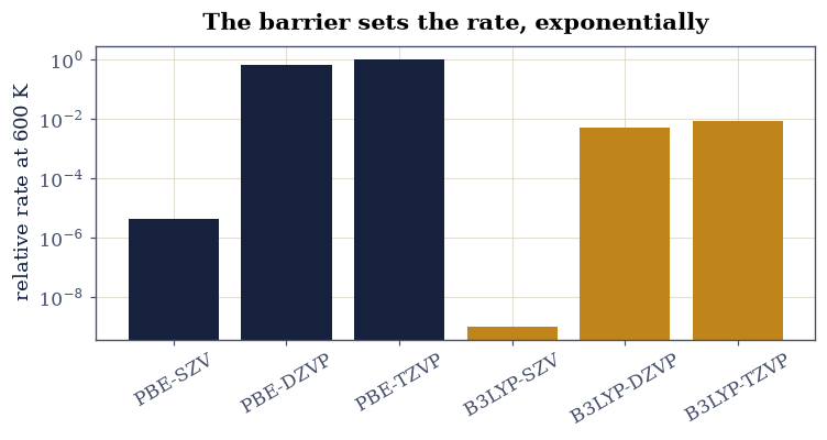
Fig. 63 Relative reaction rate \(e^{-\Delta E^{\ddagger}/k_BT}\) at 600 K (log scale) for each method, normalised to the fastest. Because the rate depends exponentially on the barrier, the few-kcal/mol differences between functionals and basis sets become many orders of magnitude in rate: a converged method is not optional.#
predicted rate varies by a factor of 9.5e+08 across the six methods at 600 K
Validation 4 — the rate spans many orders of magnitude#
Because \(k\propto e^{-\Delta E^{\ddagger}/k_BT}\), the ~25 kcal/mol spread of barriers must translate into many orders of magnitude in rate, the practical reason method convergence matters.
✓ the method choice changes the predicted rate by orders of magnitude [fastest/slowest rate = 9.5e+08 at 600 K]
True
Exercise 5 — What an experiment would actually measure#
Exercise 4 compared rates through the Boltzmann factor \(e^{-\Delta E^{\ddagger}/k_BT}\), which is enough to show that method choice matters. It is not what a kineticist measures. An experiment reports an Arrhenius activation energy, obtained by fitting
to rate constants taken over a range of temperatures, and reading \(E_a\) off the slope against \(1/T\). It is tempting to equate that \(E_a\) with the computed barrier. They are not the same number, and the difference is not experimental error.
Transition-state theory Eq. 53 carries a temperature-dependent prefactor, \(k = (k_BT/h)\,e^{-\Delta E^{\ddagger}/RT}\). Taking the logarithm and differentiating with respect to \(1/T\), that extra factor of \(T\) contributes its own slope:
So the measured activation energy sits above the computed barrier by \(RT\) — about 1.2 kcal/mol at 600 K. Small next to a 60 kcal/mol barrier, but it is a systematic offset, and comparing a computed \(\Delta E^{\ddagger}\) with a measured \(E_a\) without it is simply comparing two different quantities.
A second correction runs the other way. The reaction coordinate at a saddle point is an imaginary-frequency mode, and light nuclei tunnel through the barrier rather than only passing over it. Wigner’s leading correction multiplies the rate by
with \(|\nu^{\ddagger}|\) the magnitude of the imaginary frequency. It is always greater than one — tunnelling can only help — and it dies away as temperature rises, because a hot enough molecule does not need to tunnel.
Part a) Implement eyring_rate(barrier_kcal, T) from Eq. 53, using
scipy.constants for \(k_B\), \(h\) and \(R\) rather than typed digits. Evaluate it for
the converged B3LYP-TZVP barrier on numpy.linspace(500, 700, 41) K.
Write this one yourself — the implementation is the lesson.
Part b) Fit Eq. 54 to those rates: numpy.polyfit of \(\ln k\)
against \(1/T\), degree 1, with \(E_a = -R\times\text{slope}\). Compare \(E_a\) with the
barrier you put in, and check the difference against \(RT_0\) at the window’s mean
inverse temperature \(T_0 = 1/\langle 1/T\rangle\).
Part c) Apply Eq. 56 for an imaginary frequency of \(600\,\)cm\(^{-1}\), a representative value for a breaking C–O stretch, and report how much tunnelling changes the rate at each end of the window. Plot the Arrhenius line and the tunnelling factor together.
barrier (B3LYP-TZVP)        = 66.080 kcal/mol
Arrhenius Ea from the fit   = 67.254 kcal/mol
offset Ea - barrier         = 1.1737 kcal/mol
R*T0 at T0 = 594.1 K        = 1.1806 kcal/mol   (ratio 0.9941, theory 1)
Wigner kappa: 1.124 at 500 K -> 1.063 at 700 K
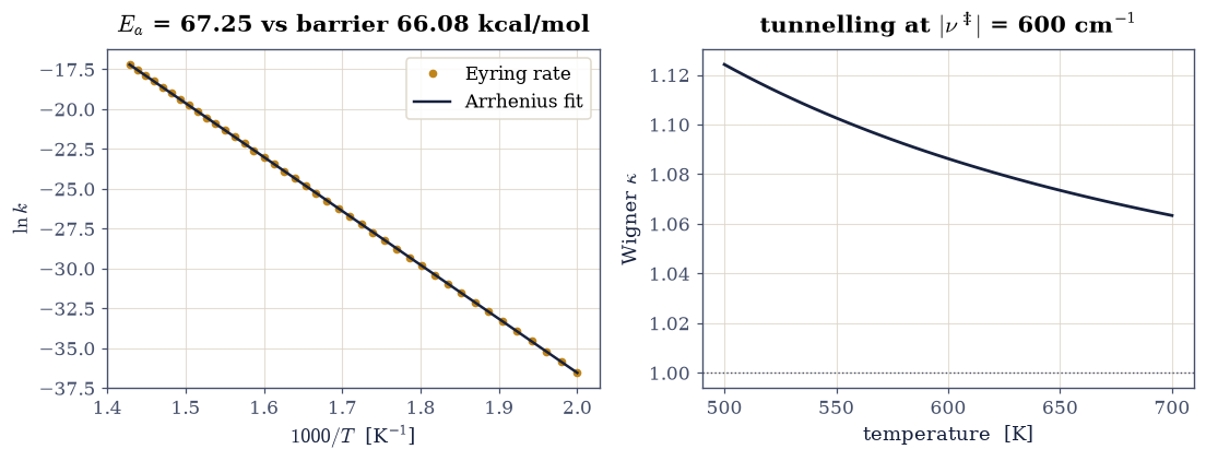
Fig. 64 Left: the Eyring rate constant for the converged B3LYP-TZVP barrier, plotted as \(\ln k\) against \(1/T\) over 500–700 K, with the straight-line Arrhenius fit. The fit is excellent, yet its slope returns an activation energy \(RT\) ABOVE the barrier that generated it – the temperature-dependent prefactor of transition-state theory contributes its own slope. Right: Wigner’s tunnelling correction \(\kappa(T)\) for an imaginary frequency of 600 cm\(^{-1}\); it exceeds one at all temperatures, since tunnelling can only speed a reaction up, and decays as thermal energy makes it unnecessary.#
Validation 5 — the measured activation energy is not the barrier#
Three checks, all deterministic. The fitted activation energy must come out above the barrier that generated the data, which is the whole point and would fail immediately if the Eyring prefactor were dropped. The size of that excess must match \(RT_0\), which is a prediction with no free parameters. And the tunnelling factor must exceed one everywhere and fall with temperature — a \(\kappa\) below one would mean tunnelling had slowed the reaction down.
✓  the Arrhenius activation energy exceeds the barrier that generated the rates: the (k_B T / h) prefactor contributes its own slope, so a measured Ea and a computed barrier are different quantities   [Ea = 67.254 vs barrier 66.080 kcal/mol]
✓  and the excess is R*T0 exactly, as eq-ea-offset predicts with no free parameters (a finite fit window averages the pointwise relation, hence the sub-percent tolerance)   [got 0.994088 vs expected 1 (rtol=0.03, atol=1e-09)]
✓  and Wigner tunnelling can only speed the reaction up, by less and less as thermal energy makes the detour unnecessary   [kappa from 1.124 at 500 K to 1.063 at 700 K]
True
Exercise 6 — The basis-set limit, extrapolated rather than bought#
Exercise 3 declared the basis “converged at TZVP” because the last step was small. There is a sharper statement available, and the committed energies have exactly the shape it needs: three basis levels per functional, SZV → DZVP → TZVP, are three points on the standard exponential approach to the complete-basis-set limit,
with three unknowns — so the extrapolation is solved, not fitted: \(r = (E_3 - E_2)/(E_2 - E_1)\), and \(E_{\rm CBS} = E_3 - (E_3-E_2)\,r/(1-r)\) sums the geometric tail. Monotone convergence (\(0 < r < 1\)) is a precondition the data must earn before the formula means anything, and the committed barriers earn it in both functional families.
The payoff is a separation of errors no single calculation can perform. The basis-set error is whatever extrapolates away; the functional error is whatever remains between PBE’s and B3LYP’s limits after it has. One number shrinks toward zero, the other survives — and only the survivor is physics.
Part a) Solve Eq. 57 for each functional family’s barrier and confirm the geometric preconditions.
Part b) Quantify the separation: the residual basis error at TZVP, and the functional gap at SZV against the functional gap at the limit.
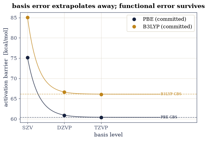
Fig. 65 The committed activation barriers against basis level for both functionals, with the three-point exponential extrapolation of Eq. eq-cbs drawn through each family to its complete-basis-set asymptote (dashed). Both families converge geometrically (0 < r < 1, checked before the formula is trusted), and both limits sit within a kcal/mol of TZVP — the quantitative form of Exercise 3’s convergence claim. What does not extrapolate away is the gap between the two asymptotes: the functional difference survives the basis limit, which is exactly what makes it a statement about the physics of the approximation rather than about the size of the expansion.#
PBE:   r = 0.037, CBS barrier 60.39 kcal/mol (TZVP residual -0.02)
B3LYP: r = 0.029, CBS barrier 66.10 kcal/mol (TZVP residual -0.02)
functional gap: 9.9 kcal/mol at SZV -> 5.7 at the basis-set limit -- the part that is physics
Validation 6 — geometric, converged, and honestly separated#
Four checks. Both families must converge geometrically — \(0 < r < 1\) is the precondition that licenses the extrapolation at all. Both limits must lie within a kcal/mol of TZVP, turning Exercise 3’s “converged” into a number. The functional gap at the limit must remain chemically large — that is the error no basis can buy away. And the SZV gap must exceed the limit gap, the direct demonstration that part of the apparent method disagreement was only basis error in disguise.
✓  both functional families converge geometrically with basis level, the precondition that makes eq-cbs an extrapolation rather than a guess   [r = 0.037 (PBE), 0.029 (B3LYP)]
✓  both CBS limits sit within a kcal/mol of TZVP: Exercise 3's convergence claim, now with the remaining error quantified rather than declared small   [TZVP residuals -0.02 and -0.02 kcal/mol]
✓  the PBE-B3LYP gap survives the basis-set limit at chemical size: the functional difference is physics, not expansion artefact   [limit gap 5.7 kcal/mol]
✓  and the apparent method disagreement at SZV was partly basis error in disguise: the gap shrinks by several kcal/mol on the way to the limit   [gap 9.9 (SZV) -> 5.7 (CBS) kcal/mol]
True
Notebook summary#
We assembled the reaction profile for ethanol dehydration from the course’s committed PBE and B3LYP energies. Every method gave a positive barrier over a transition state with a stretched C–O bond and an endothermic reaction, and the barrier converged with basis-set size: the minimal SZV overshoots, while DZVP and TZVP agree, the converged B3LYP-TZVP barrier of \(66\,\)kcal/mol landing in the experimental range. Because the rate depends exponentially on the barrier, the few-kcal/mol spread between methods becomes orders of magnitude in predicted rate, so method convergence is not optional.
Outlook#
The full path. A nudged-elastic-band calculation (next notebook) finds the transition state and the minimum-energy path, rather than assuming a single TS geometry.
Free energy, not just energy. Adding vibrational entropy gives the activation free energy \(\Delta G^{\ddagger}\) and the absolute Eyring prefactor \(k_BT/h\), hence an actual rate in s⁻¹.
Dispersion and exact exchange. B3LYP’s admixture of exact exchange improves barriers; adding a dispersion correction (D3) matters more for larger molecules.
Catalysis. The gas-phase barrier here is large; an acid catalyst opens a lower path, the reason the reaction is run over a catalyst in practice.
References#
Axel D. Becke. Density-functional thermochemistry. III. the role of exact exchange. The Journal of Chemical Physics, 98(7):5648–5652, 1993. doi:10.1063/1.464913.
John P. Perdew, Kieron Burke, and Matthias Ernzerhof. Generalized gradient approximation made simple. Physical Review Letters, 77(18):3865–3868, 1996. doi:10.1103/PhysRevLett.77.3865.