4.2 The Formation of Molecular Oxygen

Molecular and Materials Modelling

Volume IV — Electronic Structure Notebook 4.2

Why oxygen is magnetic, read from a real CP2K calculation: the electron density and the charge that builds up on bonding, the molecular orbitals themselves, and the spin-split eigenvalues that put two unpaired electrons in the π* orbitals and make O₂ a triplet.

Based on FS 2023 · Lecture 6 (molecular orbital theory)

Level · intermediate   •   Est. · 90–120 min

Raymond Amador v1.2.0  ·  2026-07-27  ·  CC BY 4.0 (text) / MIT (code)

Notebook overview

This exercise examines the formation of triplet oxygen, the most stable and most common form of O₂. Triplet oxygen has two electrons in its two degenerate \(\pi^*\) orbitals, and according to Hund’s rules the configuration with those two electrons unpaired, with parallel spins, is the one nature chooses: the total spin is \(S=1\), a triplet, and the molecule is magnetic. A simple Lewis structure, with every electron paired, misses this entirely. Molecular-orbital theory does not, and it is the molecular-orbital picture we build and verify here.

We work from a real Hartree-Fock calculation. The course ran O₂ in CP2K, printing the electron density and the frontier molecular orbitals to cube files, and we use that genuine output: we visualise the electron density, compute the density difference that shows where charge moves when the bond forms, look at the molecular orbitals one by one, repeat for the single oxygen atom, and finally read the spin-split eigenvalues from the run to build the molecular-orbital schema and explain the paramagnetism.

Provenance. This notebook develops Lecture 6 of the course (the formation of molecular oxygen via molecular-orbital theory), an exercise designed by the author (Raymond Amador), and follows its assignments. The cube visualisations and eigenvalues are the real CP2K output of the exercise (an anonymised course run), with the volumetric cubes downsampled for size; the input deck shown is the course’s own. The full course credit is in the footer.

Reading a validation. Each task closes with a check against an independent fact: electron conservation, the electron count of the molecule versus the atom, the spin imbalance that defines the triplet. A ✗ flags a mismatch to track down, not a verdict; a ✓ is strong evidence, not proof.

Scope. Cube data are visualised as isosurfaces; energies are converted from Hartree to eV. For the chemistry see Atkins & Friedman [AF11]; the calculations were run in CP2K; the cube format stores a scalar field on a 3-D grid.

Theory in brief

From atomic orbitals to molecular orbitals

When two atoms bond, their atomic orbitals combine into molecular orbitals: an in-phase bonding combination, lower in energy, with charge piled up between the nuclei, and an out-of-phase antibonding combination (starred), higher in energy, with a node between them. For O₂ the valence \(2s\) and \(2p\) orbitals build the set

(39)\[\sigma_{2s},\ \sigma_{2s}^{*},\ \sigma_{2p},\ \pi_{2p}\,(\times 2),\ \pi_{2p}^{*}\,(\times 2),\ \sigma_{2p}^{*},\]

the two \(\pi_{2p}\) and the two \(\pi_{2p}^{*}\) each a degenerate pair. Oxygen brings six valence electrons each, twelve in all, which fill the diagram from the bottom and leave the last two electrons in the degenerate \(\pi^*\) pair.

Spin, and the triplet

Two electrons in two equal orbitals follow Hund’s rule: one in each, spins parallel, because same-spin electrons keep apart (Pauli) and so repel less. The spins do not cancel (\(S=1\)), the molecule is a triplet, and it is paramagnetic, with a spin-only moment \(\mu=\sqrt{n(n+2)}\,\mu_B\) for \(n\) unpaired electrons. A spin-polarised calculation makes this concrete by solving for spin-up (\(\alpha\)) and spin-down (\(\beta\)) electrons separately: the two unpaired \(\pi^*\) electrons are both \(\alpha\), so the molecule has two more \(\alpha\) electrons than \(\beta\), the numerical fingerprint of the triplet that we will read straight off the eigenvalues.

What the calculation gives us

Hartree-Fock in CP2K returns the electron density \(\rho(\mathbf r)\), the individual molecular orbitals \(\psi_i(\mathbf r)\), and their energies \(\varepsilon_i\), written to cube files (a scalar on a 3-D grid) and to the output log. Subtracting the densities of the separated atoms from the molecule gives the density difference, a direct picture of the bond; the orbital cubes show the \(\sigma\) and \(\pi\) shapes themselves; and the eigenvalues, split by spin, build the molecular-orbital schema.

---

Setup

The Setup below holds this notebook’s data and instruments — nothing you are asked to build. It is collapsed so the building stays yours; expand it whenever you want the details.

Show code cell source

Hide code cell source

import os

import numpy as np
import matplotlib.pyplot as plt
import matplotlib.colors as mcolors
import scipy.ndimage as ndi
from mpl_toolkits.mplot3d.art3d import Poly3DCollection
from skimage.measure import marching_cubes

from ecp import validate

INK, AMBER, SOFT = "#16213e", "#c0851a", "#46506b"
from scipy.constants import physical_constants

# data: unit conversions for the committed CP2K output. The cube reader and the
# isosurface plotter below are instruments — parsing a volumetric file format and
# drawing a contour are not the lesson of a molecular-orbital notebook. The model
# that PREDICTS what those files show is the lesson, and it is built in Exercise 7.
HARTREE_EV = physical_constants["Hartree energy in eV"][0]
BOHR_A = physical_constants["Bohr radius"][0] * 1e10  # Bohr radius in Å


def data_file(name):
    """Locate a shipped data file, from the repo root (CI) or the notebook dir (Colab).

    Parameters
    ----------
    name : str
        File name (or relative path) under a ``data`` directory.

    Returns
    -------
    str
        The first existing path found.

    Raises
    ------
    FileNotFoundError
        If the file is not found under any candidate base.
    """
    for base in ("data", os.path.join("notebooks", "04-electronic-structure", "data")):
        path = os.path.join(base, name)
        if os.path.exists(path):
            return path
    raise FileNotFoundError(name)


def read_cube(name):
    """Parse a Gaussian cube file.

    Parameters
    ----------
    name : str
        Cube file name.

    Returns
    -------
    dict
        Keys: ``label``, ``origin`` (3,), ``vec`` (3, 3) voxel vectors, ``atoms``
        (n_at, 3) coordinates, ``data`` the 3-D scalar grid, and ``dV`` the
        voxel volume.
    """
    lines = open(data_file(name)).read().splitlines()
    label = lines[0].strip()
    n_at = int(lines[2].split()[0])
    origin = np.array(lines[2].split()[1:4], float)
    vec = np.array([[float(x) for x in lines[3 + i].split()[1:4]] for i in range(3)])
    ng = [int(lines[3 + i].split()[0]) for i in range(3)]
    atoms = np.array(
        [[float(x) for x in lines[6 + i].split()[2:5]] for i in range(n_at)]
    )
    data = np.array(" ".join(lines[6 + n_at :]).split(), float).reshape(ng)
    return dict(
        label=label,
        origin=origin,
        vec=vec,
        atoms=atoms,
        data=data,
        dV=abs(np.linalg.det(vec)),
    )


def add_isosurfaces(ax, cube, levels, upsample=3, alpha=1.0):
    """Draw a cube file's isosurfaces on a 3-D axis, lit and depth-sorted.

    The committed cubes are downsampled to keep the repository lean, and a
    marching-cubes mesh built directly on that coarse grid renders as large flat
    facets. The field itself is smooth, so a cubic-spline interpolation of the
    grid (display only — every integral in this notebook is computed on the raw
    committed data) recovers a mesh close to what the full-resolution cube would
    give. All levels go into a single collection so matplotlib's painter sort
    sees every triangle at once, and faces are shaded by their normals against a
    fixed light, which is what makes the lobes read as three-dimensional.

    Parameters
    ----------
    ax : mpl_toolkits.mplot3d.axes3d.Axes3D
        The target 3-D axis.
    cube : dict
        A parsed cube from ``read_cube``.
    levels : list of tuple
        ``(isovalue, colour)`` pairs (amber for positive lobes, navy for negative).
    upsample : int, optional
        Spline upsampling factor for the display mesh (default 3).
    alpha : float, optional
        Surface opacity. Opaque suits well-separated orbital lobes; a density
        that encloses its nucleus, or a difference density whose two signs
        interpenetrate, needs some translucency to show what is inside.

    Returns
    -------
    numpy.ndarray
        All surface vertices, shape (n, 3) — the caller frames the view with them.
    """
    d, vec, origin = cube["data"], cube["vec"], cube["origin"]
    spacing = (vec[0, 0], vec[1, 1], vec[2, 2])
    dz = ndi.zoom(d, upsample, order=3)
    sp = tuple(s * (n - 1) / (nz - 1) for s, n, nz in zip(spacing, d.shape, dz.shape))
    light = np.array([0.45, 0.3, 0.85])
    light = light / np.linalg.norm(light)
    tris, cols, all_verts = [], [], []
    for lvl, col in levels:
        if not (dz.min() < lvl < dz.max()):
            continue
        verts, faces, _, _ = marching_cubes(dz, level=lvl, spacing=sp)
        verts = verts + origin
        tri = verts[faces]
        normal = np.cross(tri[:, 1] - tri[:, 0], tri[:, 2] - tri[:, 0])
        normal = normal / (np.linalg.norm(normal, axis=1, keepdims=True) + 1e-30)
        # two-sided lighting: a closed lobe shows both face orientations
        shade = 0.62 + 0.38 * np.abs(normal @ light)
        base = np.array(mcolors.to_rgb(col))
        rgb = np.clip(shade[:, None] * base[None, :], 0.0, 1.0)
        tris.append(tri)
        cols.append(np.concatenate([rgb, np.full((len(rgb), 1), alpha)], axis=1))
        all_verts.append(verts)
    if tris:
        coll = Poly3DCollection(
            np.concatenate(tris), facecolors=np.concatenate(cols), edgecolor="none"
        )
        ax.add_collection3d(coll)
    return np.concatenate(all_verts) if all_verts else np.zeros((0, 3))


def frame_molecule(ax, verts, atoms, title):
    """Frame a 3-D axis tightly around a rendered molecule.

    The default framing shows the whole simulation cell, most of which is vacuum,
    so the molecule shrinks into a corner of an empty box. Fitting the limits to
    the surface and the atoms — with the same span on every axis, so nothing is
    distorted — is what makes the orbital fill the figure.

    Parameters
    ----------
    ax : mpl_toolkits.mplot3d.axes3d.Axes3D
        The target 3-D axis.
    verts : numpy.ndarray
        Surface vertices from :func:`add_isosurfaces`, shape (n, 3).
    atoms : numpy.ndarray
        Atom positions, shape (n_atoms, 3).
    title : str
        Panel title.
    """
    ax.scatter(
        *atoms.T, s=110, color="#3a3a3a", edgecolor="white", lw=1.0, depthshade=False
    )
    pts = np.vstack([verts, atoms]) if len(verts) else atoms
    centre = 0.5 * (pts.min(axis=0) + pts.max(axis=0))
    # Per-axis limits, with the box aspect set to the same ratios: units stay
    # equal on screen (nothing is distorted), but an elongated molecule gets an
    # elongated box instead of rattling around inside a cube of vacuum.
    span = pts.max(axis=0) - pts.min(axis=0)
    half = 0.56 * np.maximum(span, 0.45 * span.max())
    ax.set_xlim(centre[0] - half[0], centre[0] + half[0])
    ax.set_ylim(centre[1] - half[1], centre[1] + half[1])
    ax.set_zlim(centre[2] - half[2], centre[2] + half[2])
    ax.set_box_aspect(tuple(half))
    # The cubes put the molecular axis along z; rolling the camera by 90 degrees
    # lays it horizontal on screen, the orientation every textbook MO diagram
    # uses, and the one that actually fills a wide panel.
    ax.view_init(elev=12, azim=-58, roll=90)
    ax.set_axis_off()
    ax.set_title(title)


def show_isosurface(cube, levels, title, alpha=1.0):
    """Render cube isosurfaces with the atoms marked, on a new 3-D figure.

    Parameters
    ----------
    cube : dict
        A parsed cube from ``read_cube``.
    levels : list of tuple
        ``(isovalue, colour)`` pairs (amber for positive lobes, navy for negative).
    title : str
        Figure title.

    Returns
    -------
    matplotlib.figure.Figure
        The figure with the rendered isosurface(s).
    """
    fig = plt.figure(figsize=(4.8, 4.5))
    ax = fig.add_subplot(projection="3d")
    verts = add_isosurfaces(ax, cube, levels, alpha=alpha)
    frame_molecule(ax, verts, cube["atoms"], title)
    fig.subplots_adjust(left=0.0, right=1.0, bottom=0.0, top=0.92)
    return fig

Exercise 1 — The CP2K input file

Every calculation starts from its input deck. The course’s triplet.inp is a spin-polarised (LSD) Hartree-Fock run with the triplet imposed through MULTIPLICITY 3 (so \(2S+1=3\), \(S=1\)), and a &PRINT block that writes the cube files we will use:

&DFT
  LSD                       ! spin-polarised: separate alpha and beta densities
  MULTIPLICITY 3            ! triplet (two unpaired electrons)
  &PRINT
    &E_DENSITY_CUBE         ! write the electron density to a cube file
    &END E_DENSITY_CUBE
    &MO_CUBES               ! write molecular-orbital cubes
      NHOMO -1              ! ... every occupied MO (HOMO down)
      NLUMO 3               ! ... and three lowest unoccupied
    &END MO_CUBES
  &END PRINT
&END DFT

It ships with this notebook: triplet.inp. Those two print directives are exactly what generate the density and orbital cubes the rest of the exercise visualises.

Part a) Read the deck.

Part b) Confirm it requests a triplet and the cube output.

MULTIPLICITY = 3  ->  S = 1 (triplet); writes density cube: True

Validation 1 — the deck describes a triplet with cube output

The input must specify multiplicity 3 (a spin-1 triplet) and request the electron density cube, the two ingredients the rest of the exercise depends on.

✓  the input deck requests a triplet (multiplicity 3) and writes the density cube   [MULTIPLICITY = 3 (S = 1), E_DENSITY_CUBE = True]

True

Exercise 2 — The electron density

Once the job finishes it writes the electron density to a cube file: the scalar \(\rho(\mathbf r)\) on a 3-D grid. We render it as an isosurface, the surface on which the density takes a chosen value, with the two oxygen nuclei marked. The density is a single smooth cloud enveloping both atoms, the hallmark of a bound molecule rather than two separate ones.

Part a) Read and render the O₂ electron-density cube.

Part b) Confirm it is a physical density.

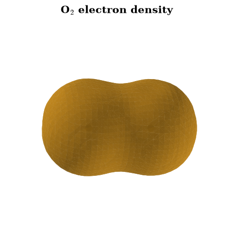
Fig. 44 Isosurface of the O₂ electron density from the CP2K calculation (amber, \(\rho=0.05\,e/a_0^3\)), with the two oxygen nuclei marked. The density forms a single connected cloud spanning both atoms, the signature of a bonded molecule. (Cube downsampled for display.)

min ρ = -8.76e-06; ∫ρ d³r = 11.885 (the 12 GTH valence electrons)

Validation 2 — a physical electron density

A real electron density is non-negative everywhere. (The integral under-counts here only because the cube was downsampled for size, blurring the sharp peaks at the nuclei; we check the electron count properly in Exercises 3 and 5.)

✓  the electron density is non-negative everywhere (to numerical noise)   [min ρ = -8.76e-06, max ρ = 0.946]

True

Exercise 3 — The density difference (Assignment 1)

The total density is striking but not the most informative quantity; the difference is. Subtracting the densities of the two separate oxygen atoms from the molecule’s density, \(\Delta\rho=\rho_{\mathrm{O_2}}-\rho_{\mathrm{O}}-\rho_{\mathrm{O}}\), isolates exactly the charge that rearranges when the bond forms: amber where electrons accumulate, navy where they are depleted. Because the molecule and the two atoms hold the same total number of electrons, the difference must integrate to zero, which is our check.

Part a) Render the density-difference cube.

Part b) Confirm electron number is conserved.

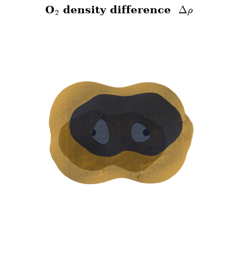
Fig. 45 Electron-density difference \(\Delta\rho=\rho_{\mathrm{O_2}}-2\rho_{\mathrm{O}}\) from the CP2K calculation: amber where charge accumulates on bonding, navy where it is depleted (\(\pm0.004\,e/a_0^3\)). The redistribution into the bonding region is what a Lewis double bond depicts only schematically. (Cube downsampled for display.)

Validation 3 — electron conservation

Forming a bond moves charge around but neither creates nor destroys it, so the density difference must integrate to ≈ 0.

✓  the density difference integrates to zero (electrons conserved)   [got -0.0194206 vs expected 0 (rtol=1e-06, atol=0.05)]

True

Exercise 4 — The molecular orbitals (Assignment 2)

The calculation also prints individual molecular orbitals. Their cube file names encode which orbital each is: a comment line reads WAVEFUNCTION i spin s i.e. HOMO - n, so the highest occupied (the HOMO) is \(n=0\), the one below it \(n=1\), and so on. Decoding those tags identifies three valence orbitals worth seeing: a bonding \(\pi_{2p}\), a bonding \(\sigma_{2p}\), and the antibonding \(\pi^*\) that is the HOMO and holds the two unpaired electrons. Bonding orbitals concentrate charge between the nuclei; the antibonding \(\pi^*\) has a node there, visible as the change of lobe colour across the bond.

Part a) Render the three orbitals.

Part b) Confirm they are proper (normalised) one-electron orbitals.

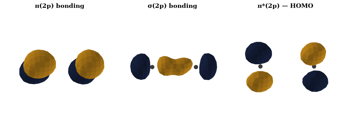
Fig. 46 Three O₂ molecular orbitals from the CP2K calculation (amber/navy = opposite sign of the wavefunction): the bonding \(\pi_{2p}\) and \(\sigma_{2p}\), which build up amplitude between the nuclei, and the antibonding \(\pi^*\) (the HOMO), whose node between the atoms is the colour change across the bond. The two electrons in this \(\pi^*\) pair are the unpaired ones. (Cubes downsampled for display.)

∫|ψ|² d³r = 0.9870, 0.9994, 1.0200

Validation 4 — proper one-electron orbitals

Each Hartree-Fock orbital is normalised, so \(\int|\psi|^2\,dV\) must be the same for all three (the same value the downsampling preserves), confirming they are genuine single-electron molecular orbitals.

✓  the three orbitals share one normalisation (∫|ψ|² equal)   [max|Δ| = 0.0329698 (rtol=0.05, atol=1e-09)]

True

Exercise 5 — The oxygen atom (Assignment 3)

The same calculation for a single oxygen atom gives a reference. Its density is one spherical-ish cloud about a single nucleus, and crucially it holds half the electrons of the molecule. Comparing the integrated densities is a clean, downsampling-proof check: the molecule must contain exactly twice the atom’s electrons — 12 valence electrons against 6, since the GTH pseudopotentials fold each 1s core into the potential and the cubes therefore hold valence density only — so the ratio of the integrals is 2, with the per-cent-level shortfall of each absolute integral being the coarse grid’s quadrature error.

Part a) Render the O-atom density.

Part b) Confirm the molecule has twice the atom’s electrons.

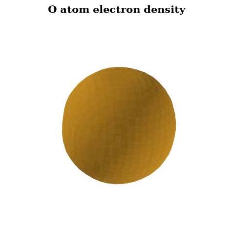
Fig. 47 Electron density of a single oxygen atom from the CP2K calculation (amber, \(\rho=0.05\,e/a_0^3\)): one cloud about one nucleus, holding its six valence electrons — the 1s core is folded into the GTH pseudopotential — half the molecule’s twelve. (Cube downsampled for display.)

∫ρ(O₂) = 11.89, ∫ρ(O) = 5.95 valence electrons  ->  ratio 1.998  (12 vs 6; the 1s cores live in the pseudopotential)

Validation 5 — the molecule has twice the atom’s electrons

The ratio of the integrated densities must be 2: the molecule is two oxygen atoms’ worth of electrons.

✓  O₂ holds twice the electrons of an O atom (integral ratio = 2)   [got 1.99767 vs expected 2 (rtol=0.03, atol=1e-09)]

True

Exercise 6 — The eigenvalues and the molecular-orbital schema (Assignment 4)

Finally we read the energies. The output lists the occupied eigenvalues separately for spin-up (\(\alpha\)) and spin-down (\(\beta\)), and the asymmetry is the whole story: there are nine occupied \(\alpha\) orbitals but only seven occupied \(\beta\), a difference of two. Those two extra spin-up electrons sit in the degenerate \(\pi^*\) pair with no spin-down partners, exactly the unpaired electrons of the triplet. Dropping the two core \(1s\) states, we plot the valence levels at their real energies and fill them with \(\alpha\) (up) and \(\beta\) (down) electrons, reproducing the molecular-orbital schema from the calculation itself.

One feature departs from the idealised diagram of Eq. 39: in the spin-up (\(\alpha\)) channel the bonding \(\pi_{2p}\) pair sits just below \(\sigma_{2p}\), because the two unpaired \(\alpha\) electrons in \(\pi^*\) exchange-stabilise the same-spin bonding \(\alpha\,\pi_{2p}\). The spin-down (\(\beta\)) channel, with \(\pi^*\) empty, keeps the textbook \(\sigma_{2p}\)-below-\(\pi_{2p}\) order. Either way the last two electrons occupy the \(\pi^*\) pair, so the triplet conclusion is unchanged.

Part a) Build the schema from the real eigenvalues.

Part b) Confirm the spin imbalance, and the paramagnetic moment it implies.

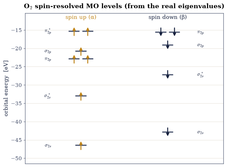
Fig. 48 Spin-resolved molecular-orbital levels of O₂ from the real CP2K eigenvalues (valence only; the two 1s cores omitted), each level drawn at its own energy: spin-up (α, amber) on the left, spin-down (β, navy) on the right. The α channel fills seven levels — including both π* orbitals — while β fills only five, its π* empty; those two unpaired α electrons in π* are the triplet ground state and the origin of O₂’s paramagnetism. The exchange asymmetry the text describes shows too: the α bonding-π pair sits just below α σ, while β keeps the textbook σ-below-π order.

occupied: 9 α, 7 β  ->  2 unpaired electrons; μ = 2.83 μ_B

Validation 6 — two unpaired electrons, a paramagnetic triplet

The spin-up/spin-down imbalance must be exactly two unpaired electrons, giving spin \(S=1\) and the spin-only moment \(\mu=\sqrt{8}\approx2.83\,\mu_B\): O₂ is a paramagnetic triplet, the result a Lewis structure cannot give.

✓  O₂ has two unpaired electrons (S=1) and a non-zero magnetic moment   [2 unpaired → μ = 2.83 μ_B]

True

Exercise 7 — The model that predicts the triplet

Everything so far has been read from a calculation. That is the honest way to treat density-functional theory, which no notebook can reimplement — but it leaves a question standing. Did we need the calculation to know O₂ is a triplet?

We did not, and the model that gets there is old enough to predate quantum chemistry software entirely. Take one \(2s\) and three \(2p\) orbitals on each atom and let each pair combine into a bonding and an antibonding molecular orbital. For two atomic orbitals of the same energy \(\alpha\) coupled by a resonance integral \(\beta\) with overlap \(S\), the secular problem gives

(40)\[E_{\pm} = \frac{\alpha \pm \beta}{1 \pm S},\]

with \(\beta<0\), so \(E_+\) lies below \(\alpha\) and \(E_-\) above it. The overlap in the denominator is what makes the antibonding orbital rise more than the bonding one falls, which is why filling both is worse than filling neither. Two \(p\) orbitals pointing at each other overlap head-on and split strongly (\(\sigma\)); the two perpendicular pairs overlap sideways and split weakly (\(\pi\)), and stay degenerate with each other by symmetry.

Fill the resulting ladder with O₂’s twelve valence electrons under the Aufbau principle and Hund’s rule, and the last two land in the degenerate \(\pi^*\) pair with parallel spins. That is the triplet — obtained from symmetry, counting and one \(2\times2\) secular equation, with no self-consistent field anywhere.

Part a) Implement two_centre(alpha, beta, overlap) returning the bonding and antibonding pair of Eq. 40. Confirm on the way that the antibonding orbital is destabilised by more than the bonding one is stabilised, which is the whole reason a filled antibonding level cancels more than a bond. Write this one yourself — the implementation is the lesson.

Part b) Assemble the valence ladder: \(\sigma_{2s}\), \(\sigma^*_{2s}\) from the \(2s\) pair, and \(\sigma_{2p}\), \(\pi_{2p}\) (twofold), \(\pi^*_{2p}\) (twofold), \(\sigma^*_{2p}\) from the \(2p\) set. Fill twelve electrons with numpy bookkeeping, applying Hund’s rule within the degenerate \(\pi^*\) level: singly occupy both before pairing either.

Part c) Read off the bond order \((n_{\rm bonding}-n_{\rm antibonding})/2\) and the number of unpaired electrons, and compare both with the calculation. The model owes nothing to the CP2K output, so agreement here is a genuine cross-check of the picture against the machine.

filled levels: [('sigma_2s', 2), ('sigma*_2s', 2), ('sigma_2p', 2), ('pi_2p', 4), ('pi*_2p', 2)]
bonding 8, antibonding 4  ->  bond order 2.0
unpaired electrons predicted by LCAO+Hund: 2
unpaired electrons measured from the CP2K output (Exercise 6): 2

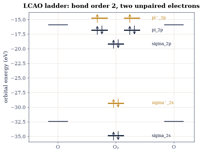
Fig. 49 The LCAO molecular-orbital ladder of O₂ built from Eq. eq-lcao-two-centre, with the atomic \(2s\) and \(2p\) levels of each oxygen at the sides and the molecular levels between them. Bonding levels are drawn in navy, antibonding in amber; arrows show the twelve valence electrons filled by Aufbau, with Hund’s rule leaving one electron in each of the degenerate \(\pi^*\) orbitals. Bond order two and two unpaired electrons follow from counting alone – the same conclusion the committed density-functional calculation reaches in Exercise 6.

Validation 7 — the picture agrees with the machine

The model is checked on the two things it actually claims, both of them integers that follow from symmetry and counting rather than from the illustrative parameter values: a bond order of two, and two unpaired electrons. The second is then set against the spin imbalance measured from the committed CP2K eigenvalues in Exercise 6 — two calculations with nothing in common but the physics.

✓  the antibonding level rises further than the bonding level falls, the asymmetry the overlap denominator of eq-lcao-two-centre puts there   [up +1.122 eV vs down -0.918 eV]
✓  filling the LCAO ladder with 12 valence electrons gives bond order 2, the double bond of O₂   [got 2 vs expected 2 (rtol=1e-12, atol=1e-09)]
✓  and Hund's rule in the degenerate pi* pair predicts exactly the two unpaired electrons the density-functional calculation reports: the picture and the machine agree   [LCAO predicts 2, CP2K output gives 2]

True

Exercise 8 — The deck reproduced: unrestricted Hartree–Fock, live

Everything above analyses the committed CP2K output. This exercise closes the loop by running the deck’s calculation, here and now: the committed input specified XC_FUNCTIONAL NONE with MULTIPLICITY 3 and LSD — unrestricted Hartree–Fock with two more α than β electrons — and PySCF can do exactly that in under a second. Two runs, triplet and singlet, and three verdicts to read.

First the ordering: the triplet must fall below the singlet, Hund’s rule as an energy difference rather than a slogan — with the standing caveat that the singlet of O\(_2\) is genuinely multireference, so its single-determinant energy is only good enough to order, never to quote. Second, the spin: an unrestricted determinant is not an eigenstate of \(\hat S^2\), and the measured \(\langle S^2\rangle\) lands slightly above the exact \(S(S+1) = 2\) — that excess is spin contamination, the price UHF pays for letting α and β orbitals differ, and reading its size is part of reading any unrestricted calculation. Third, the pattern: the α/β occupation structure must match the committed CP2K eigenvalue schema of Exercise 6 — nine α against seven β valence electrons, with the β LUMO a degenerate π\(^\ast\) pair, the two holes Hund’s rule carved out.

Part a) Run UHF for the triplet and the singlet at the experimental bond length and report total energies and \(\langle S^2\rangle\).

Part b) Read the three verdicts: ordering, contamination, and the α/β level pattern against the committed CP2K schema.

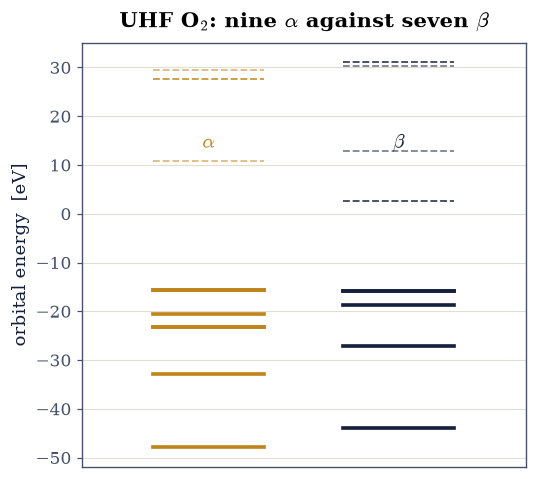
Fig. 50 The valence orbital energies of triplet O2 from the live unrestricted Hartree–Fock run, α spin channel (amber) against β (navy), each level drawn at its computed energy. The two channels agree on the deep σ levels, then part company where the physics lives: the α channel holds the degenerate π* pair as its highest occupied levels, while in the β channel that same pair is empty — the two unpaired electrons of the triplet, in the same nine-against-seven pattern as the committed CP2K eigenvalues of Exercise 6. The dashed markers show the empty β π* pair, degenerate to machine precision.

E(triplet) = -149.545575 Ha, E(singlet) = -149.513527 Ha  ->  triplet lower by 0.87 eV
<S^2> = 2.0334 (exact S(S+1) = 2; the excess 0.0334 is UHF spin contamination)
occupations: 9 alpha / 7 beta; beta LUMO pair split 1.97e-15 Ha -- the two degenerate pi* holes of Exercise 6's committed schema

Validation 8 — the deck’s physics, recomputed and re-verdicted

Four checks. Both SCF runs must have converged, or nothing downstream means anything. The triplet must lie below the singlet — Hund’s rule as an energy difference, ordering only, the singlet being multireference. The spin contamination must be positive and small: \(\langle S^2\rangle\) just above 2 is the signature of a mildly spin-broken unrestricted triplet, and a large excess would indict the calculation. And the α/β pattern must reproduce the committed CP2K schema — two more α than β, with the empty β π\(^\ast\) pair degenerate to machine precision, since that degeneracy is symmetry rather than fitting.

✓  both unrestricted SCF runs converged   [triplet True, singlet True]
✓  the triplet lies well below the single-determinant singlet: Hund's rule as a computed energy difference, ordering gated and the singlet's multireference character left honestly unquoted   [triplet below by 0.87 eV]
✓  the spin contamination is positive and small: <S^2> sits just above the exact 2, the fingerprint of a mildly spin-broken UHF triplet   [<S^2> - 2 = 0.0334]
✓  and the alpha/beta structure reproduces the committed CP2K schema: two more alpha electrons than beta, and the beta LUMO a pi* pair degenerate to machine precision -- the two holes Hund's rule carved   [9 alpha / 7 beta; beta-LUMO split 2.0e-15 Ha]

True

Notebook summary

We worked the real CP2K calculation of molecular oxygen end to end: the electron density, the bonding charge build-up in the density difference (which integrates to zero, conserving electrons), the bonding \(\pi\) and \(\sigma\) and antibonding \(\pi^*\) molecular orbitals, and the single oxygen atom for comparison. The spin-resolved eigenvalues told the central story: nine occupied \(\alpha\) orbitals against seven \(\beta\), the difference of two being the unpaired electrons in the degenerate \(\pi^*\) pair. That is why ground-state O\(_2\) is a paramagnetic triplet, the result a Lewis structure cannot give.

Outlook

• The spin density. The calculation also wrote a spin-density cube, \(\rho_\alpha-\rho_\beta\); rendering it shows the unpaired-electron density sitting exactly in the \(\pi^*\) orbitals.

• Singlet oxygen. Pairing the two \(\pi^*\) electrons gives the reactive ¹Δg state, 0.98 eV higher; it is multireference, so a single-determinant method describes it only crudely.

• The second row. B₂ is paramagnetic for the same reason, while C₂ and N₂ are not; the \(\sigma_{2p}/\pi_{2p}\) ordering switches before O₂ through s–p mixing.

• Beyond Hartree-Fock. O₂’s bond energy needs correlated methods (CCSD(T)) or good functionals; Hartree-Fock alone underbinds it badly.

References

[AF11]

Peter W. Atkins and Ronald S. Friedman. Molecular Quantum Mechanics. Oxford University Press, 5 edition, 2011.

Take this notebook with you

Use the download button (↓) in the toolbar above to save this notebook and run it yourself. The published notebooks ship without worked solutions; if you would like the reference solutions — to teach from or to check your own work — get in touch: hello@ramador.me.

Based on the lecture and exercise materials of Molecular and Materials Modelling (ETH Zürich and Empa, FS 2023), developed by Prof. Dr. Daniele Passerone (lectures), Dr. Carlo Pignedoli, and the author (exercises); here synthesised, expanded, and restyled by the author.