


1.2 Lattice-Gas Monte Carlo and Kinetic Monte Carlo#
Notebook overview#
Where notebook 1.1 put a spin on every lattice site, here each site is either empty or holds an adsorbed molecule, and the molecules attract their neighbours: the lattice gas, the canonical model of adsorption, wetting, and island growth on surfaces. We study it on a honeycomb lattice (each site has three neighbours), the geometry of many molecular adlayers, and we simulate it in two complementary ways.
First, equilibrium Metropolis Monte Carlo: the same accept/reject rule as in 1.1, used here to sample adsorbate configurations, measure how clustering grows with the binding energy, and estimate a dimer binding energy from cluster statistics. We pin the sampler down against an exact enumeration of a small lattice and against the ideal-gas (non-interacting) limit, which has a closed-form answer. Second, kinetic Monte Carlo (KMC): the residence-time algorithm that advances physical time by sampling Poisson-distributed waiting times, turning the model into a movie of diffusion-limited aggregation.
Provenance. This notebook also develops Lecture 2 (the foundations of Monte Carlo): Dr. Carlo Pignedoli’s lattice-gas and kinetic-Monte-Carlo exercise, here redesigned and rephrased by the author, reimplemented cleanly, and restyled; the full course credit is in the footer.
Reading a validation. Each exercise ends with a check against something independent: an exact enumeration, the ideal-gas combinatorics, the Poisson statistics the algorithm is built on. A ✗ is a prompt to locate a discrepancy (a real error, a convention, or Monte Carlo noise against a tight tolerance), not an automatic verdict; a ✓ is strong evidence, not proof.
Units and scope. Energies (binding energy, barriers) and temperature are in the same arbitrary unit, so \(k_B=1\) and \(\beta=1/T\). This is a working review; for the methods see Newman & Barkema [NB99], Frenkel & Smit [FS02], and, for kinetic Monte Carlo, Voter’s primer [Vot07] and the original Bortz–Kalos–Lebowitz [BKL75] and Gillespie [Gil77] algorithms.
Theory in brief#
The lattice-gas model#
Put an occupation variable \(n_i\in\{0,1\}\) on every site \(i\) of a honeycomb lattice (\(M=2L^2\) sites, coordination number \(z=3\)). Occupied nearest neighbours lower the energy by the binding energy \(\,d_e<0\):
the sum running over nearest-neighbour bonds. The control parameters are the binding energy \(d_e\), the temperature \(T\), and the coverage
(The lattice gas is exactly equivalent to the Ising model of 1.1 under \(n_i=(\sigma_i+1)/2\); we keep the occupation language because it matches the physics of adsorption.)
Sampling equilibrium: Metropolis Monte Carlo#
To sample configurations with Boltzmann weight \(P\propto e^{-\beta E}\) we reuse the Metropolis rule from 1.1: propose a move, compute its energy change \(\Delta E\), and accept it with probability \(\min(1,e^{-\beta\Delta E})\), which satisfies detailed balance. The natural move for a fixed number of molecules is to pick an occupied site and a random empty site and attempt to move the molecule there; only the bonds at the old and new positions change, so \(\Delta E\) is local. Metropolis samples equilibrium: it has no notion of time.
Sampling dynamics: kinetic Monte Carlo#
Real surface processes happen at rates. An activated event \(k\) (a hop, a bond formation) over a barrier \(E_k\) occurs with an Arrhenius rate
\(\nu\) an attempt frequency. The kinetic Monte Carlo (residence-time, or Bortz–Kalos–Lebowitz) algorithm samples the master equation exactly: at each step it lists every possible event with its rate, forms the total rate
picks one event with probability \(r_k/R\), executes it, and advances the clock by a waiting time drawn from the exponential (Poisson) distribution with mean \(1/R\),
Unlike Metropolis, KMC produces a trajectory in real time: it is how one simulates diffusion-limited growth, catalysis, and dewetting.
Setup#
The Setup below holds this notebook’s data and instruments — nothing you are asked to build. It is collapsed so the building stays yours; expand it whenever you want the details.
Exercise 1 — The honeycomb lattice and the adsorbate model#
Build the lattice and the two quantities every later exercise needs: the number of occupied nearest-neighbour pairs and, through Eq. 15, the energy. The schematic shows the geometry (two interleaved sublattices, each site bonded to three neighbours) with one molecule and the three neighbours whose occupancy sets its contribution to the energy.
Part a) Confirm the lattice is what it claims to be: every one of the
\(2L^2\) sites has exactly three neighbours, the neighbour relation is symmetric
(if \(i\) lists \(j\) then \(j\) lists \(i\)), and the lattice is bipartite, with the A
sublattice coupling only to B. Use collections.Counter over the neighbour lists
rather than a spot check — a lattice builder that is wrong at the periodic seam
is right almost everywhere.
Part b) Check the energy bookkeeping of Eq. 15: an isolated molecule contributes no pairs, and one adjacent pair contributes exactly one bond of energy \(d_e\). Getting this wrong by a factor of two is the single most common lattice-model error, because each bond is reachable from both of its ends.
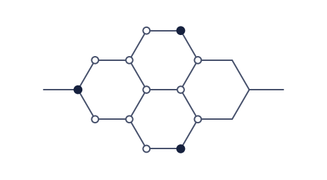
Fig. 13 A patch of the honeycomb adsorption lattice: open circles are empty sites of the two sublattices, joined by nearest-neighbour bonds (grey). The amber molecule occupies one site; the three navy molecules are its nearest neighbours, the only sites whose occupancy enters its bond energy \(d_e\sum_{\langle ij\rangle} n_i n_j\) (Eq. eq-lg-energy).#
coordination numbers: {3: 18} (every site must have 3)
neighbour relation symmetric: True; A couples only to B: True
isolated molecule: 0 pairs; adjacent pair: 1 pair -> energy d_e, not 2 d_e
Validation 1 — the energy bookkeeping#
Two molecules placed on adjacent sites must register exactly one occupied pair
(energy \(d_e\)); two molecules far apart must register none. This pins down
n_pairs and the meaning of Eq. 15.
✓ honeycomb has z=3 with a symmetric, bipartite neighbour relation, and the pair count books one bond per adjacent pair [adjacent→1 pair, isolated→0 pairs]
True
Exercise 2 — Equilibrium Metropolis Monte Carlo, checked by exact enumeration#
A Metropolis move picks an occupied site and a random empty site and attempts to move the molecule there, accepting with \(\min(1,e^{-\beta\Delta E})\) where \(\Delta E\) counts only the bonds gained and lost. The cleanest possible test is a lattice small enough to solve exactly: for \(L=2\) (\(M=8\) sites) with \(N=3\) molecules there are only \(\binom{8}{3}=56\) configurations, so the Boltzmann average \(\langle E\rangle\) can be summed directly. A correct sampler must reproduce it.
Part a) Implement metropolis_sweep(occ, occupied, nbr, de, beta, n_moves),
proposing n_moves single-molecule hops to a random empty site and accepting each
with probability \(\min(1, e^{-\beta\Delta E})\). Compute \(\Delta E\) from the change
in pair count local to the move — the moved molecule’s old and new neighbours —
never by re-evaluating the whole lattice, which would turn an \(O(z)\) update into
an \(O(N)\) one.
Write this one yourself — the implementation is the lesson.
Part b) Run it on the \(L=2\) lattice and compare \(\langle E\rangle\) with the exact enumeration over all \(\binom{8}{N}\) configurations. At this size the exact answer is available, which is the only reason the sampler can be proved right rather than merely made plausible.
Validation 2 — sampler vs. exact enumeration#
The Monte Carlo average energy must match the exact Boltzmann sum on the small lattice: the decisive check that the move samples the correct ensemble.
✓ MC ⟨E⟩ matches exact enumeration (L=2, N=3) [got -0.08392 vs expected -0.0837896 (rtol=0.05, atol=1e-09)]
True
Exercise 3 — The ideal lattice gas (\(d_e=0\))#
Switch off the interaction. With \(d_e=0\) every configuration is equally likely, so the molecules are placed at random and the expected number of occupied nearest-neighbour pairs is a pure combinatorial fact: each of the \(N_{\rm bonds}\) bonds is occupied at both ends with probability \(\binom{M-2}{N-2}/\binom{M}{N}\), giving
This non-interacting baseline \(\langle N_{\rm pairs}\rangle_0\) is exactly the reference we need for the binding-energy estimate in the next exercise.
Part a) Run the sampler at \(d_e = 0\), where the molecules are non-interacting and every arrangement of \(N\) molecules on \(2L^2\) sites is equally likely.
Part b) Compare the measured mean pair count with the combinatorial prediction Eq. 20. This is a check on the sampler, not on the physics: at \(d_e = 0\) the answer is pure counting, so any disagreement indicts the Metropolis implementation rather than the model.
Validation 3 — the ideal-gas combinatorics#
With no interaction the measured pair count must equal the random-placement prediction Eq. 20, the sampler reproducing the analytic ideal-gas limit.
✓ d_e=0 pair count matches the ideal-gas combinatorics [got 1.90067 vs expected 1.90141 (rtol=0.05, atol=1e-09)]
True
Exercise 4 — Binding energy, clustering, and a dimer binding-energy estimate#
Turn the interaction back on. As \(d_e\) becomes more negative, attraction pulls molecules together and the number of occupied pairs grows, the lattice gas clusters. This is the basis of a classic experimental trick: measure the dimer concentration \(n\) in the interacting system and the non-interacting baseline \(n_0\) (Eq. 20), and invert the dilute-limit law-of-mass-action relation \(n/n_0\sim e^{-\beta d_e}\) to read off the binding energy,
We test the whole chain by a round trip: choose a true \(d_e\), simulate to get \(n\), take \(n_0\) from \(d_e=0\), and check that Eq. 21 recovers \(d_e\). It is only a rough estimate (the dilute-limit derivation drops correlations), so we expect the right sign and order of magnitude, not three digits. The animation shows molecules diffusing and aggregating as the sampler equilibrates.
Part a) Scan the binding energy \(d_e\) and show the mean pair count rising as the interaction is turned on — clustering, measured rather than asserted.
Part b) Invert the measurement: form the dimer estimate Eq. 21 from the observed pair counts and compare it with the \(d_e\) that was fed in. A round trip through the model that returns its own input is a far stronger statement than a monotonic trend.
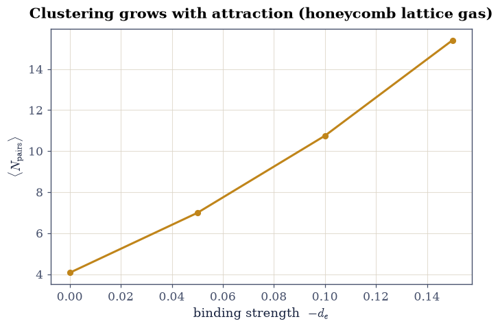
Fig. 14 Clustering of the honeycomb lattice gas: the mean number of occupied nearest-neighbour pairs \(\langle N_{\rm pairs}\rangle\) (coverage \(\theta=0.15\), \(T=0.06\)) rises monotonically with the binding strength \(-d_e\), as attraction draws the adsorbates together.#
Validation 4 — clustering trend and the binding-energy round trip#
Two checks: the pair count must increase monotonically as the attraction strengthens, and the rough estimate Eq. 21 must recover the input \(d_e\) to within a factor of two (right sign and order of magnitude).
✓ clustering grows monotonically as binding strengthens [⟨pairs⟩ at d_e=[np.float64(0.0), np.float64(-0.05), np.float64(-0.1), np.float64(-0.15)] → [4.1, 7.0, 10.7, 15.4]]
✓ kT·ln(n0/n) recovers the binding energy to within a factor of ~2 [d_e(true)=-0.100, estimate=-0.058]
True
Watching the lattice gas equilibrate#
Starting from a random placement at a clustering binding energy, the Metropolis dynamics pull the molecules into compact islands as the run proceeds.
Fig. 15 Animation of equilibrium Metropolis Monte Carlo for the honeycomb lattice gas at coverage \(\theta=0.15\), \(d_e=-0.15\), \(T=0.06\): from a random initial placement the molecules (amber) diffuse and aggregate into compact islands as the sampler approaches the Boltzmann distribution.#
Exercise 5 — Kinetic Monte Carlo: the residence-time algorithm#
Metropolis told us where equilibrium sits; KMC tells us how fast the system gets there. The algorithm rests on two statistical guarantees, and we verify both directly. Given a catalogue of events with rates \(r_k\) and total rate \(R\) (Eq. 18): (i) each step advances physical time by an exponentially distributed waiting time of mean \(1/R\) (Eq. 19), so \(\langle\Delta t\rangle=1/R\) and, for an exponential law, the standard deviation equals the mean; (ii) the executed event is chosen with probability proportional to its rate, \(r_k/R\).
Part a) Draw many waiting times for a fixed total rate \(R\) using Eq. 19, and check both the mean and the spread against the exponential distribution: \(\langle\Delta t\rangle = 1/R\) and \(\sigma_{\Delta t} = 1/R\) too. The standard deviation equalling the mean is the signature of a Poisson process, and checking only the mean would miss a wrong distribution with the right average. Write this one yourself — the implementation is the lesson.
Part b) Select many events from a fixed rate catalogue and confirm the selection frequencies track the rates in proportion. Together the two parts are the algorithm’s whole correctness claim: when the next event happens, and which one it is.
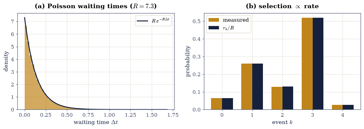
Fig. 16 The two statistical guarantees of the residence-time KMC algorithm: (a) the waiting times \(\Delta t=-\ln\rho/R\) for fixed total rate \(R=7.3\) follow the exponential law \(R\,e^{-R\Delta t}\) (mean and standard deviation both \(1/R\)); (b) over many steps each event \(k\) is executed with frequency equal to \(r_k/R\).#
Validation 5 — the two guarantees of the algorithm#
The waiting-time mean and standard deviation must both equal \(1/R\) (the exponential signature), and the event frequencies must match \(r_k/R\).
✓ KMC waiting-time mean equals 1/R [got 0.136917 vs expected 0.136986 (rtol=0.02, atol=1e-09)]
✓ KMC waiting time is exponential (std = mean) [got 0.137384 vs expected 0.136986 (rtol=0.03, atol=1e-09)]
✓ KMC selects events with frequency proportional to rate [max|Δ| = 0.00059974 (rtol=0.03, atol=0.003)]
True
Exercise 6 — Diffusion-limited growth#
Now run the algorithm. Molecules start mobile and randomly placed; each mobile molecule can diffuse to an empty neighbour at rate \(r_d=\nu e^{-\beta E_d}\) or, if it touches another molecule, bind irreversibly at rate \(r_b=\nu e^{-\beta E_b}\) (Eq. 17). The clock advances by Eq. 19 after every event. From a well-mixed start the molecules diffuse, meet, and freeze into growing clusters: diffusion-limited aggregation, played out in real time.
Part a) Implement kmc_step(occ, nbr, r_d, r_b): build the rate catalogue
for the current configuration, draw the waiting time from Eq. 19,
select an event with the residence-time rule of Exercise 5, and execute it.
Every step advances physical time by a different amount — that is the whole
difference between kinetic Monte Carlo and the Metropolis sweeps of Exercise 2,
whose steps carry no time at all.
Write this one yourself — the implementation is the lesson.
Part b) Run it from a random start, recording snapshots, and confirm that aggregation has occurred: the mean cluster size must rise well above the random-start baseline. Compare against that baseline rather than against zero, since a random configuration already contains adjacent pairs by chance.
Fig. 17 Animation of kinetic Monte Carlo diffusion-limited growth on the honeycomb lattice (\(\theta=0.30\), equal diffusion and binding barriers \(E_d=E_b=0.1\), \(T=0.1\)): mobile molecules (amber) diffuse until contact, then bind irreversibly (navy), so compact and branched frozen clusters grow out of the well-mixed initial gas.#
Validation 6 — aggregation has occurred#
Diffusion-limited growth must turn the well-mixed start (clusters of size ≈ 1–2) into substantially larger aggregates: the mean cluster size must exceed the random baseline by a clear margin.
✓ KMC growth aggregates the gas into larger clusters [mean cluster size 1.66 → 2.90, largest = 11, elapsed t = 65.9]
True
Exercise 7 — Rejection-free bookkeeping, and the clock made physical#
Exercise 6’s stepper is honest and slow: it re-enumerates every molecule’s options at every step, so each event costs \(O(N)\) work even though the event itself touches a handful of sites. The production form of the algorithm — Bortz–Kalos–Lebowitz [BKL75] — keeps the event catalogue alive between steps: executing an event can only change the options of the sites whose neighbourhood it altered, so only those entries are recomputed. Same process, same distributions, a fraction of the work.
The second half of the exercise cashes the cheque the residence-time clock has been writing all along. For a single tracer on the empty honeycomb lattice the diffusivity is exact: every hop goes to one of three neighbours chosen uniformly and independently of history, so consecutive hop vectors are uncorrelated, \(\langle r^2\rangle = n\,a^2\) after \(n\) hops with \(a\) the bond length, and each hop waits an exponential time of mean \(1/r_d\). In two dimensions \(\langle r^2\rangle = 4Dt\), so
and measuring \(D(T)\) from trajectories must hand back the barrier \(E_d\) the rates were built from — the model’s own closed loop, and the demonstration that kMC time is physical time once \(\nu\) is given a value.
Part a) Implement the BKL bookkeeping: an event dictionary
site -> (can_hop, can_bind) refreshed only on the sites an executed event
touched. Write this one yourself — the implementation is the lesson.
Certify it the strongest way available: after every step of a full run,
compare the live dictionary against a from-scratch enumeration of the current
configuration. Set equality, not statistics — and note what it buys: if the
catalogue is identical at every configuration and the selection uses the same
rates, the two steppers sample identical processes, so no distributional
comparison is needed afterwards.
Part b) Measure the work. The naive stepper provably scans every mobile molecule each step (its loop is the proof), so its cost on a trajectory is the mobile count; the BKL cost is the number of refreshed sites. Plot both along a growth run and report the ratio.
Part c) Run the tracer. Measure \(\langle r^2\rangle/n\) against the exact \(a^2\), measure \(D\) at three temperatures, and fit the Arrhenius slope of \(\ln D\) against \(1/T\) — it must return \(E_d\). Then attach numbers: with \(\nu = 10^{13}\,\)s\(^{-1}\) and \(a = 2.46\,\)Å, report \(D\) in cm\(^2\)/s.
certification: 0 catalogue mismatches over 242 steps (run ended with every molecule frozen or isolated)
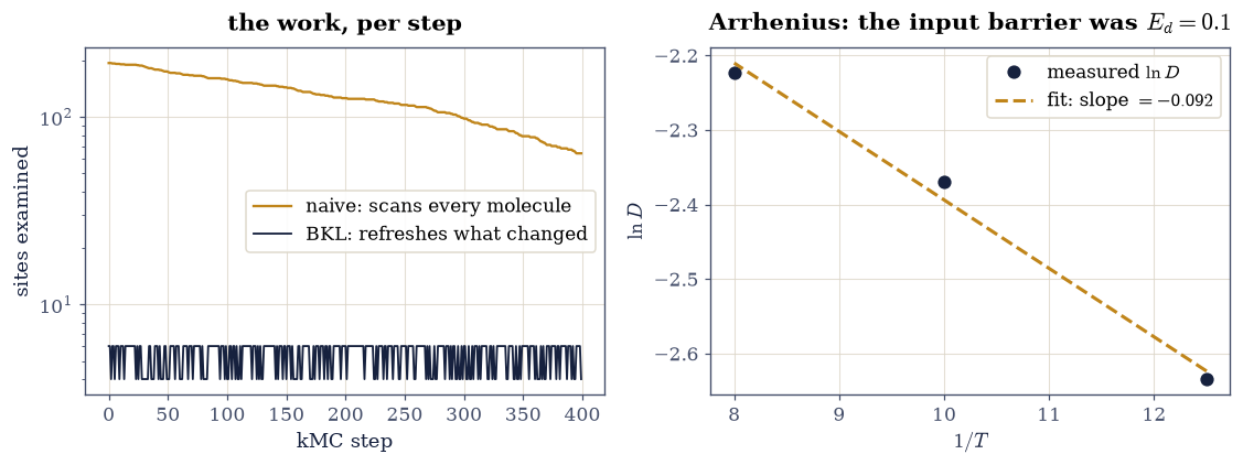
Fig. 18 Left: work per kinetic Monte Carlo step along a growth run, measured as sites examined — the naive stepper re-scans every mobile molecule (amber), the BKL stepper refreshes only the neighbourhood the executed event touched (navy), and the gap is the algorithmic content of Bortz–Kalos–Lebowitz. Right: the tracer diffusivity against inverse temperature on Arrhenius axes; the fitted slope returns the input diffusion barrier, closing the loop between the microscopic rates the simulation was built from and the transport coefficient it predicts, Eq. eq-kmc-tracer.#
work ratio naive/BKL over the growth run: 24.0x
tracer <r^2>/n = 1.0031 (exact 1); mean wait x rate = 1.0011 (exact 1); D(T=0.08) / exact = 1.0020
Arrhenius slope returns E_d = 0.0919 (input 0.1); with nu = 1e13/s and a = 2.46 A, D(kT = 0.025 eV) = 2.77e-05 cm^2/s
Validation 7 — exact bookkeeping, measured savings, the barrier returned#
Five checks. The BKL catalogue must equal the from-scratch enumeration after every step of a full run — zero mismatches, which is bookkeeping correctness proved at the data-structure level and the reason no statistical cross-check of observables is needed. The measured work ratio must be large, since that saving is the algorithm’s entire purpose. The tracer’s squared displacement per hop must land on the exact bond length squared — via a segment estimator, because a single endpoint r² has order-one relative noise — which simultaneously certifies the uncorrelated-walk argument of Eq. 22 and the periodic unwrapping; the clock factor is gated separately and far more tightly, since a hundred thousand waiting-time draws pin it to a third of a percent. And the Arrhenius fit must hand back the diffusion barrier the rates were built from — the closed loop between microscopic input and measured transport.
✓ the live BKL catalogue equals the from-scratch enumeration after every step of a full run: the incremental bookkeeping is exact, so both steppers sample identical processes by construction [0 mismatches over 242 steps]
✓ and the saving is what the algorithm exists for: an order of magnitude less work per step on the same trajectory [naive/BKL work ratio = 24.0]
✓ the tracer's mean squared displacement per hop equals the bond length squared, as the uncorrelated-hop argument behind eq-kmc-tracer requires -- and any periodic-unwrapping error would land exactly here (segment estimator: ~1900 independent samples) [got 1.00306 vs expected 1 (rtol=0.1, atol=1e-09)]
✓ the clock factor separately: the mean exponential waiting time times the rate is 1, the residence-time algorithm's defining property, measured on a hundred thousand draws [got 1.00105 vs expected 1 (rtol=0.03, atol=1e-09)]
✓ the assembled diffusivity lands on the exact r_d a^2/4 of eq-kmc-tracer [got 0.07177 vs expected 0.0716262 (rtol=0.12, atol=1e-09)]
✓ and the Arrhenius slope of the measured diffusivity returns the input diffusion barrier: kMC time is physical time, closed loop [got 0.0918548 vs expected 0.1 (rtol=0.25, atol=1e-09)]
True
Notebook summary#
We mapped adsorption onto a honeycomb lattice gas and studied it two complementary ways. Equilibrium Metropolis Monte Carlo reproduced the exact enumerated \(\langle E\rangle\) for small systems and, with an attractive nearest-neighbour interaction, drove clustering beyond the ideal-gas coverage. Kinetic Monte Carlo with residence-time selection then advanced the same model in real time from its rate constants, producing diffusion-limited growth — first with an honest rebuild-everything stepper, then with the Bortz–Kalos–Lebowitz bookkeeping that refreshes only what an event touched, certified exact against the from-scratch catalogue at every step and twenty-four times cheaper. The clock closed the loop: a tracer’s measured diffusivity landed on the exact \(r_d a^2/4\) and its Arrhenius slope handed back the input barrier, so kMC time is physical time. The contrast is the lesson: the equilibrium and kinetic pictures answer different questions (the final structure versus the pathway and timescale that reach it) from one set of energetics.
Outlook#
Dendritic vs. compact morphology. Whether diffusion-limited growth yields ramified (dendritic) or compact islands is set by the ratio of binding to edge-diffusion rates. Capturing the crossover quantitatively needs a coordination-dependent diffusion barrier (a molecule with more bonds is harder to move, \(E_d\to E_d + k\,\Delta\) for \(k\) occupied neighbours), so that slow binding lets molecules edge-diffuse into high-coordination pockets before freezing. Add that term and watch the islands compact as \(E_b\) rises above \(E_d\).
Reversible binding. Give the bound state a finite unbinding rate obeying detailed balance; the growth then anneals toward the equilibrium islands of Exercise 4, connecting the kinetic and equilibrium pictures.
Rejection-free efficiency. The event list here is rebuilt each step; the Bortz–Kalos–Lebowitz [BKL75] and binning strategies update it incrementally for large lattices.
Real time scales. Restoring physical attempt frequencies \(\nu\sim10^{12}\, \mathrm{s^{-1}}\) in Eq. 17 turns the dimensionless clock into seconds, letting KMC bridge to experimental deposition rates.
References#
A. B. Bortz, M. H. Kalos, and J. L. Lebowitz. A new algorithm for monte carlo simulation of ising spin systems. Journal of Computational Physics, 17(1):10–18, 1975. doi:10.1016/0021-9991(75)90060-1.
Daan Frenkel and Berend Smit. Understanding Molecular Simulation: From Algorithms to Applications. Academic Press, 2 edition, 2002.
Daniel T. Gillespie. Exact stochastic simulation of coupled chemical reactions. The Journal of Physical Chemistry, 81(25):2340–2361, 1977. doi:10.1021/j100540a008.
M. E. J. Newman and G. T. Barkema. Monte Carlo Methods in Statistical Physics. Oxford University Press, Oxford, 1999.
Arthur F. Voter. Introduction to the kinetic monte carlo method. Radiation Effects in Solids (NATO Science Series), 235:1–23, 2007. doi:10.1007/978-1-4020-5295-8_1.