


5.2 Hydrocarbons on Platinum#
Notebook overview#
Platinum is the workhorse of catalysis, and catalysis begins with adsorption: a molecule must stick to the surface before it can react. How strongly it sticks, the adsorption energy, is the single most important number, and for hydrocarbons on a metal it depends heavily on van der Waals (dispersion) attraction, the weak, long-range force that ordinary density functionals describe poorly. This exercise makes that failure concrete.
We take the course’s optimised structures of benzene, methane, and ethane on a Pt(111) slab, and its committed total energies, and compute the adsorption energy \(E_{\rm ads}=E_{\rm mol+slab}-E_{\rm slab}-E_{\rm mol}\). We compare it across two dispersion-aware methods (the BEEF-vdW functional and the Grimme D3 correction) and against experiment, and find the central lesson of the exercise: the choice of functional moves the adsorption energy by more than an electron-volt, with one method underbinding to the point of not binding the alkanes at all, and the other overbinding.
Provenance. This notebook develops Lecture 8 of the course (adsorption energies and dispersion on Pt(111)), an exercise designed by the author (Raymond Amador). The slab and adsorption structures (
pt_slab.xyz,benzene_on_pt.xyz, …) and the total energies are the course’s own committed CP2K results (an anonymised course run); the comparison table reproduces the exercise’s. The full course credit is in the footer.
Reading a validation. Each task closes with a check against an independent fact: a real calculation’s adsorption energy against the measured one, the known ordering of binding strengths, the size of the dispersion effect. A ✗ flags a mismatch; a ✓ is strong evidence, not proof.
Scope. Energies are the committed density-functional totals (Hartree, converted to eV); we analyse them rather than recompute the slab calculations, which are large and beyond a notebook. For dispersion see Grimme’s D3 [GAEK10] and the BEEF-vdW functional [WLMogelhoj+12].
Theory in brief#
Adsorption energy#
The adsorption energy is the energy released when an isolated molecule binds to a clean surface,
negative for a bound state. Each of the three terms is a separate total-energy calculation; the adsorption energy is a small difference of three large numbers, so it demands consistency and care.
Physisorption and the van der Waals problem#
Saturated hydrocarbons have no dangling bonds, so they do not form strong chemical bonds to platinum; they physisorb, held by van der Waals attraction. This force comes from correlated electron fluctuations, which a local or semi-local functional (LDA, PBE) does not contain, so plain functionals get physisorption badly wrong. Two fixes appear here: the Grimme D3 correction adds an empirical \(-C_6/r^6\) term atom-by-atom, and the BEEF-vdW functional builds a non-local correlation term into the functional itself. They do not agree, and neither matches experiment exactly: adsorption energies remain a hard test of electronic-structure methods.
Setup#
The Setup below holds this notebook’s data and instruments — nothing you are asked to build. It is collapsed so the building stays yours; expand it whenever you want the details.
import matplotlib.colors as mcolors
from matplotlib.patches import Circle

# Ball-and-stick display radii (Å), scaled for legibility rather than physical.
DISPLAY_R = {"H": 0.44, "C": 0.78, "O": 0.74, "Pt": 1.42}


def _blend(color, f):
    """Blend a colour toward white (f>0) or black (f<0) by fraction |f|.

    Parameters
    ----------
    color : str
        Any Matplotlib colour.
    f : float
        Fraction in [-1, 1]: positive lightens, negative darkens.

    Returns
    -------
    tuple
        An (r, g, b) triple.
    """
    c = np.array(mcolors.to_rgb(color))
    target = 1.0 if f >= 0 else 0.0
    return tuple(c + (target - c) * abs(f))


def draw_structure(ax, els, xyz, view):
    """Orthographic ball-and-stick render of an atomic structure.

    Atoms are shaded spheres drawn back-to-front (a painter's algorithm) with a
    depth-faded metal substrate; bonds within the adsorbate (the non-Pt atoms)
    are drawn as sticks. This is far clearer than a 3-D scatter, which projects
    every atom to a flat disc with unreliable front-to-back occlusion.

    Parameters
    ----------
    ax : matplotlib.axes.Axes
        A 2-D axes; its aspect is set equal so the atoms stay round.
    els : list of str
        Element symbols, one per atom.
    xyz : numpy.ndarray, shape (N, 3)
        Cartesian coordinates in Å.
    view : {"side", "top"}
        "side" projects onto x-z (line of sight along y); "top" projects onto
        x-y (line of sight down z, the surface normal).
    """
    hor, ver, dep = (0, 2, 1) if view == "side" else (0, 1, 2)
    depth = xyz[:, dep]
    lo = depth.min()
    span = max(depth.max() - lo, 1e-6)
    is_mol = np.array([e != "Pt" for e in els])

    mol = np.where(is_mol)[0]
    for a in mol:
        for b in mol:
            if b <= a or np.linalg.norm(xyz[a] - xyz[b]) >= 1.7:
                continue  # C-C ~1.4 Å, C-H ~1.1 Å; longer pairs are not bonded
            zmid = ((xyz[a, dep] + xyz[b, dep]) / 2 - lo) / span
            ax.plot(
                [xyz[a, hor], xyz[b, hor]],
                [xyz[a, ver], xyz[b, ver]],
                color="#3f3f3f",
                lw=2.6,
                solid_capstyle="round",
                zorder=200 + zmid * 50,
            )

    for i in np.argsort(depth):  # far first, so near atoms occlude correctly
        el = els[i]
        base = CPK.get(el, "#888888")
        near = (xyz[i, dep] - lo) / span  # 0 far, 1 near the viewer
        if el == "Pt":
            base = _blend(base, 0.55 * (1.0 - near))  # deeper layers recede
        r = DISPLAY_R.get(el, 0.6)
        zo = (250 if is_mol[i] else 100) + near * 40
        cx, cy = xyz[i, hor], xyz[i, ver]
        ax.add_patch(
            Circle((cx, cy), r, facecolor=base, edgecolor="#20242c", lw=0.5, zorder=zo)
        )
        ax.add_patch(
            Circle(
                (cx - 0.32 * r, cy + 0.32 * r),
                0.40 * r,  # highlight
                facecolor=_blend(base, 0.6),
                edgecolor="none",
                zorder=zo + 0.1,
            )
        )

    pad = 1.6
    ax.set_xlim(xyz[:, hor].min() - pad, xyz[:, hor].max() + pad)
    ax.set_ylim(xyz[:, ver].min() - pad, xyz[:, ver].max() + pad)
    ax.set_aspect("equal")
    ax.set_xticks([])
    ax.set_yticks([])
    for spine in ax.spines.values():
        spine.set_visible(False)
Exercise 1 — The adsorption system#
The course built the adsorption geometry with ASE: a five-layer Pt(111) slab, 180 atoms, with the molecule placed above it and the whole thing relaxed. We render the committed benzene-on-Pt(111) structure, the slab a metallic raft and the flat benzene ring lying parallel just above it, the orientation that maximises its contact with the metal.
Part a) Render the benzene-on-Pt(111) system in two orthographic views: a side view showing the five stacked Pt layers and the vacuum gap, and a top view down the surface normal showing the flat benzene ring over the Pt(111) lattice. Part b) Confirm the molecule sits in a vacuum gap above the slab (a surface, not a bulk calculation).
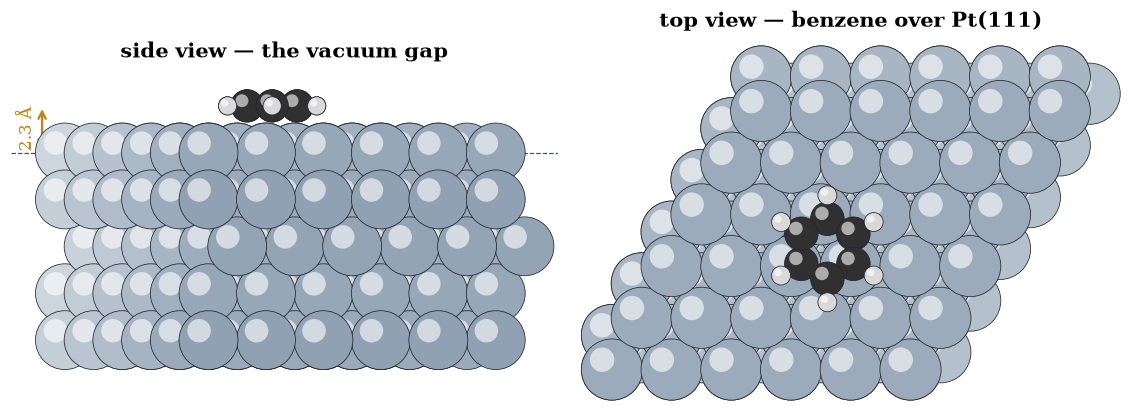
Fig. 56 The committed benzene-on-Pt(111) adsorption system, drawn as shaded spheres sorted by depth. Left, a side view: five Pt(111) layers (silver, deeper layers receding) with the benzene molecule (carbon dark, hydrogen light, bonds drawn) lying flat in the vacuum gap about 2 Å above the top layer — a surface calculation, not a bulk one. Right, a top view down the surface normal: the ring lies parallel to the metal, its whole face in contact, centred over the hexagonal Pt lattice whose lower layers show through the threefold hollows.#
benzene sits 2.25 Å above the top Pt layer (180 Pt + 12 molecule atoms)
Validation 1 — a molecule above a surface#
This must be a surface calculation: the molecule sits in the vacuum a couple of ångström above the topmost platinum layer, not buried in it.
✓ benzene sits in the vacuum gap above the Pt surface [molecule-to-surface height = 2.25 Å]
True
Exercise 2 — The adsorption energy of benzene#
The adsorption energy is the difference of three committed total-energy calculations Eq. 49: the bare slab, the isolated molecule, and the combined system. Below are the course’s committed totals (Hartree) for benzene on Pt(111). Their difference, converted to eV, is the adsorption energy, and it lands close to the experimental \(-1.7\,\)eV: benzene binds strongly, its whole \(\pi\)-face in contact with the metal. Read that agreement with care, though — Exercise 3 recomputes the adsorption energy with two different functionals and finds it moving by more than an electron-volt, so this close match is one calculation’s result, not a sign that the method is exact.
Part a) Compute \(E_{\rm ads}\) from the three totals.
Part b) Confirm this committed calculation lands near the measured benzene adsorption energy.
E_ads(benzene) = (-21748.964 − -38.177 − -21710.724) Ha × 27.21
             = -1.70 eV   (experiment -1.72 eV)
Validation 2 — benzene binds at the measured strength#
The adsorption energy from the real totals must be bound (negative) and close to the experimental \(-1.7\,\)eV.
✓ this committed calculation lands near the measured benzene adsorption energy [got -1.70172 vs expected -1.72 (rtol=1e-06, atol=0.4)]
True
Exercise 3 — Functional sensitivity (Assignment 6)#
Now the heart of the exercise. The course computed the adsorption energy of all three hydrocarbons with two dispersion-aware methods, the BEEF-vdW functional and the Grimme D3 correction, and compared them to experiment. The result is sobering: the two methods straddle the measured values, BEEF-vdW underbinding so badly that it leaves methane and ethane unbound (positive adsorption energy), and Grimme D3 overbinding every molecule. The lesson is that for physisorption the dispersion treatment, not just the functional, decides the answer.
Part a) Plot the adsorption energies of the three hydrocarbons for both methods against experiment.
Part b) Confirm dispersion is decisive: benzene binds most strongly throughout, and the two methods bracket experiment.
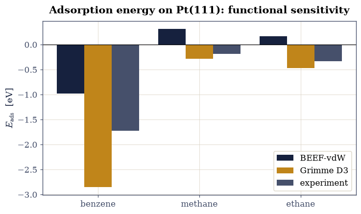
Fig. 57 Adsorption energies of benzene, methane, and ethane on Pt(111) from the course’s committed results: the BEEF-vdW functional (navy) and the Grimme D3 correction (amber) against experiment (grey). Benzene binds far more strongly than the alkanes in every method. BEEF-vdW underbinds so severely that methane and ethane come out unbound (positive); Grimme D3 overbinds. The spread, well over an electron-volt for benzene, is the functional sensitivity the exercise is named for.#
benzene binds most strongly under both functionals: True
D3 and BEEF-vdW bracket experiment for every molecule: True
Validation 3 — dispersion is decisive, and benzene binds most#
Two robust facts must hold: benzene is the most strongly bound species in every method (its large \(\pi\)-face), and the two dispersion treatments bracket experiment for benzene (BEEF-vdW above, Grimme D3 below), the signature of the functional sensitivity.
✓ benzene binds most strongly, and the two methods bracket experiment [benzene: BEEF-vdW -0.975, exp -1.72, D3 -2.852 eV]
True
Exercise 4 — Basis-set superposition error, and the counterpoise cure#
The adsorption energy Eq. 49 looks unimpeachable: take the bound system, subtract the pieces. It hides a systematic error that has embarrassed a great deal of published adsorption chemistry, and Lecture 8 names it in its own title.
The trouble is that a calculation never uses a complete basis. It uses a finite set of functions attached to the atoms. When the molecule sits on the surface, the molecule’s electrons can borrow the slab’s basis functions — and the slab’s can borrow the molecule’s. Each fragment is therefore described better in the combined calculation than it was on its own, and it is described better for a reason that has nothing whatever to do with bonding. That artificial stabilisation is counted as binding. The basis-set superposition error (BSSE) makes adsorption look stronger than it is, and it is worst exactly where it is least welcome: weak physisorption, where the true binding is small enough for the artefact to rival it.
Boys and Bernardi’s counterpoise correction [BB70] removes it by refusing the asymmetry. Compute each fragment in the full dimer basis — with the partner’s basis functions present but its nuclei and electrons absent, so-called ghost functions — so that every term in Eq. 49 is evaluated in one and the same basis:
where the superscript is the basis and the subscript the system.
We cannot run that on benzene and platinum here. We can build the mechanism from scratch, in a model small enough to see all the way through: one particle in one dimension, two Gaussian wells for the two “fragments”, and a handful of Gaussian basis functions on each. Every integral is analytic. The companion Elementary Computational Physics course does the same experiment on a real hydrogen atom with real ghost Gaussians in ECP §8.18; what follows is the same effect, stripped to the point where its cause is unmistakable.
Part a) Implement matrices(basis, wells) for a basis of Gaussians
\(g_i(x)=e^{-a_i(x-c_i)^2}\): the overlap \(S_{ij}\), the kinetic matrix, and the
potential of a set of Gaussian wells. Use the Gaussian product rule — the product
of two Gaussians is a third, centred at \(P=(a_iA+a_jB)/(a_i+a_j)\) with exponent
\(p=a_i+a_j\) and prefactor \(e^{-\mu(A-B)^2}\), \(\mu=a_ia_j/p\) — so every integral is
closed-form and nothing is quadrature. Crucially, wells lists the wells present in
the potential: a basis function whose centre is not among them is a ghost,
contributing variational freedom and no attraction. That single argument is what
makes the whole experiment possible.
Write this one yourself — the implementation is the lesson.
Part b) Solve the generalised eigenvalue problem \(Hc=ESc\) with
scipy.linalg.eigh(H, S) — generalised, because Gaussians on different centres are
not orthogonal. Compute fragment \(A\)’s ground state twice: in its own basis, and in
the combined basis with \(B\)’s functions present as ghosts. The difference is the
BSSE, and by the variational principle its sign is not in doubt.
Part c) Establish the two properties that identify BSSE as an artefact rather than physics. It must vanish as the fragments separate, since functions too far away are no use to borrow. And it must shrink as the fragment’s own basis improves, since there is nothing left to borrow once a fragment is already well described. Scan both. Watch which additions help: the diagnosis is in the detail.
E(A, own basis)          = -1.38011138
E(A, dimer basis, ghost) = -1.38127085
BSSE                     = 1.159e-03  (positive: spurious stabilisation)
BSSE vs separation: [ 1.70e-03  1.16e-03  1.85e-06  7.33e-13 -8.88e-16  0.00e+00]
BSSE vs basis size ([3, 6, 9, 12]): [1.16e-03 1.23e-05 1.17e-05 3.50e-08]
fragment energy falls monotonically with basis size: [-1.380111 -1.387219 -1.387222 -1.387247]
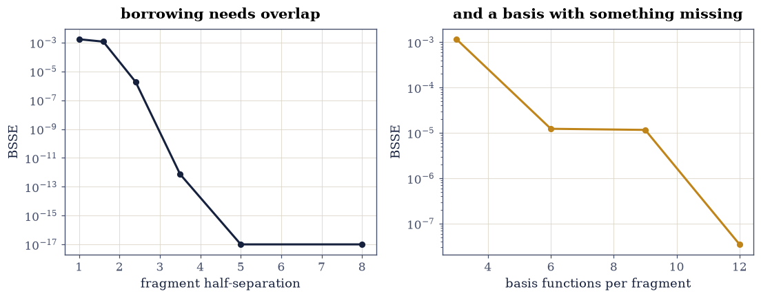
Fig. 58 Basis-set superposition error in a one-dimensional two-fragment model, computed exactly. Left: BSSE against fragment half-separation on a logarithmic axis; it falls by orders of magnitude once the fragments stop overlapping, because functions too far away cannot be borrowed. Right: BSSE against the number of basis functions per fragment; it collapses as the fragment’s own basis improves, and the collapse comes from adding a DIFFUSE exponent rather than a tight one, since it is the loosely bound tail a fragment borrows from its neighbour. Both behaviours identify BSSE as an artefact of an incomplete basis, not a property of the system.#
Validation 4 — the signature of an artefact#
Four checks, all deterministic — there is no randomness anywhere in this model, so the tolerances can be tight. The BSSE must be positive, which the variational principle guarantees and which therefore tests the implementation rather than the physics. It must fall away once the fragments stop overlapping. It must shrink as the fragment’s own basis improves. And the fragment energy itself must decrease monotonically with basis size, since adding functions can never raise a variational minimum — the check that would catch a wrong sign or a broken matrix element.
✓  ghost functions lower the fragment's energy: the variational principle guarantees the sign, so this tests the matrices rather than the physics   [BSSE = 1.159e-03]
✓  and it dies away as the fragments separate — functions too far off cannot be borrowed, which is why BSSE is a short-range artefact   [BSSE falls from 1.7e-03 at d = 1.0 to below 1e-10 by d = 3.5, decreasing at every resolvable separation]
✓  and it collapses as the fragment's own basis improves: there is nothing left to borrow once a fragment is already well described, so BSSE vanishes in the complete-basis limit   [BSSE 1.16e-03 -> 3.50e-08 for 3 -> 12 functions per fragment]
✓  the fragment energy never rises when basis functions are added, as the variational principle requires   [E = [-1.380111 -1.387219 -1.387222 -1.387247]]
True
Exercise 5 — A model of sticking: the Newns–Anderson picture#
The committed totals say how much each molecule binds; nothing yet says why an adsorbate level and a metal surface bind at all. The canonical answer is the Newns–Anderson model [New69]: one adsorbate orbital at energy \(\varepsilon_a\), hybridising with strength \(V\) into a surface band. The entire model is two functions of energy — the level broadening \(\Delta(\varepsilon) = \pi V^2 \rho_{\rm band}(\varepsilon)\) and the level shift \(\Lambda(\varepsilon)\), its Hilbert transform — and the adsorbate’s spectral function follows exactly:
where the \(\delta\)-poles are split-off states: solutions of \(\varepsilon = \varepsilon_a + \Lambda(\varepsilon)\) outside the band, where \(\Delta = 0\), each carrying weight \(w_p = [1 - \Lambda'(\varepsilon_p)]^{-1}\). For the semi-elliptic band the Hilbert transform is closed-form, so every claim below is checkable against exact limits: the sum rule (one electron of spectral weight, band plus poles, always), the wide-band limit (a Lorentzian of width \(\Delta(\varepsilon_a)\)), the threshold \(V_c = W/\sqrt2\) at which split-off states first appear for a band-centre level, and particle–hole symmetry (occupancy exactly \(\tfrac12\) at the band centre). Weak coupling is physisorption’s broadened resonance; strong coupling is chemisorption’s bonding/antibonding pair — the covalent channel this notebook’s committed, dispersion-dominated energies deliberately do not probe, built here as the instrument that would.
Part a) Implement \(\Delta\), the closed-form \(\Lambda\), the in-band \(\rho_a\), and the pole finder (searched separately below and above the band — interpolating across the gap fabricates roots). Write this one yourself — the implementation is the lesson. Gate the sum rule.
Part b) Show the two regimes and measure the threshold: scan \(V\) and find where split-off weight first appears, against the exact \(W/\sqrt2\).
Part c) Fill the level: occupancy \(n_a(\varepsilon_a)\) at fixed Fermi energy, with the exact half-filling point and the two saturation limits.
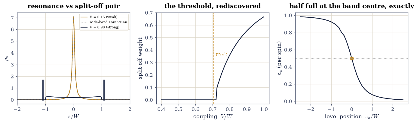
Fig. 59 The Newns–Anderson model with a semi-elliptic surface band, every panel checkable against a closed form. Left: the adsorbate spectral function in the two regimes — weak coupling gives a broadened resonance inside the band (amber, indistinguishable from the wide-band Lorentzian, dotted), strong coupling splits bonding and antibonding states off both band edges (navy sticks), the spectral picture of chemisorption. Middle: the split-off weight against coupling strength; it first appears at the exact threshold W/√2 for a band-centre level (dashed). Right: the level occupancy against level position at fixed Fermi energy — exactly one half at the band centre by particle–hole symmetry, saturating to full and empty in the deep and high limits.#
sum rule: weak 1.00000, strong 1.00000 (strong = band 0.446 + poles 0.554)
threshold: measured V_c = 0.725, exact W/sqrt(2) = 0.707
occupancy at band centre: 0.5000 (exact 1/2 by particle-hole symmetry)
Validation 5 — a model held to its own closed forms#
Five checks, every one against an exact statement of the model. The spectral weight must sum to one in both regimes — band plus poles, the sum rule that catches any error in \(\Lambda\), the pole weights, or the branch choice. The weak-coupling resonance must be the wide-band Lorentzian. The split-off threshold must land on \(W/\sqrt2\). The band-centre occupancy must be exactly one half. And the occupancy must fall monotonically as the level rises through the band — filling behaving like filling.
✓  the spectral sum rule holds in the weak-coupling regime: one electron of weight, all of it in-band   [got 1 vs expected 1 (rtol=0.001, atol=1e-09)]
✓  and in the strong-coupling regime, where over half the weight has split off the band edges -- the same electron, redistributed into the bonding/antibonding pair   [got 1 vs expected 1 (rtol=0.001, atol=1e-09)]
✓  the weak-coupling resonance is the wide-band Lorentzian of width Delta(ea), the analytic limit the full solution must contain   [L1 difference over the resonance window < 0.08]
✓  split-off states first appear at the exact threshold W/sqrt(2) for a band-centre level -- the scan rediscovers the closed form   [got 0.725 vs expected 0.707107 (rtol=1e-06, atol=0.02)]
✓  the occupancy is exactly one half at the band centre (particle-hole symmetry) and falls monotonically as the level rises through the band   [n(0) = 0.5000; monotone over 41 level positions]
True
Notebook summary#
We computed the adsorption energies of benzene, methane, and ethane on Pt(111) from the course’s committed total energies. Benzene’s \(-1.70\,\)eV from a real calculation matched the measured value, and comparing the dispersion-aware methods exposed the exercise’s point: the BEEF-vdW functional underbinds so badly it leaves the alkanes unbound, while the Grimme-D3 correction overbinds, the two bracketing experiment. For physisorbed hydrocarbons it is the van der Waals treatment, not just the functional, that decides the answer.
Outlook#
The deformation energy. Splitting \(E_{\rm ads}\) into the cost of distorting the molecule and slab into their adsorbed shapes plus the pure interaction separates geometry from binding.
Site dependence. Repeating the calculation with the molecule over a top, bridge, or hollow site maps the corrugation of the surface potential.
Coverage. Larger or smaller surface cells change the adsorbate-adsorbate spacing, giving the adsorption energy as a function of coverage.
Beyond pairwise dispersion. Many-body dispersion (MBD) and the RPA go past the pairwise \(-C_6/r^6\) picture and tend to improve metal-surface adsorption.
References#
S. F. Boys and F. Bernardi. The calculation of small molecular interactions by the differences of separate total energies. some procedures with reduced errors. Molecular Physics, 19(4):553–566, 1970. doi:10.1080/00268977000101561.
Stefan Grimme, Jens Antony, Stephan Ehrlich, and Helge Krieg. A consistent and accurate ab initio parametrization of density functional dispersion correction (DFT-D) for the 94 elements H-Pu. The Journal of Chemical Physics, 132(15):154104, 2010. doi:10.1063/1.3382344.
D. M. Newns. Self-consistent model of hydrogen chemisorption. Physical Review, 178(3):1123–1135, 1969. doi:10.1103/PhysRev.178.1123.
Jess Wellendorff, Keld T. Lundgaard, Andreas Møgelhøj, and others. Density functionals for surface science: exchange-correlation model development with Bayesian error estimation. Physical Review B, 85(23):235149, 2012. doi:10.1103/PhysRevB.85.235149.