3.2 Replica Exchange and the Melting of a Cluster

Molecular and Materials Modelling

Volume III — Molecular Dynamics Notebook 3.2

The sampling problem of rugged landscapes, the parallel-tempering algorithm that solves it by swapping configurations between temperatures, and its payoff in the real LAMMPS run of the course: the caloric curve and heat-capacity peak that locate the melting of a 38-atom argon cluster.

Based on FS 2023 · Lecture 12 (replica exchange)

Level · intermediate   •   Est. · 90–120 min

Raymond Amador v1.2.0  ·  2026-07-27  ·  CC BY 4.0 (text) / MIT (code)

Notebook overview

A single molecular-dynamics trajectory has a blind spot. On a rugged landscape, with deep minima separated by high barriers, a low-temperature run never has the energy to climb out of the basin it starts in, so its averages depend on where it began. The previous notebook met this as the trapping of an optimization; here it becomes the central problem of sampling. The fix is elegant: run many copies of the system at different temperatures at once, and let them trade configurations. The hot copies cross barriers freely, the cold copies inherit those crossings through the swaps, and the whole set samples the landscape far better than any one of them could alone. This is replica exchange, or parallel tempering.

This is the exercise from Lecture 12, and we take it in two steps. First we build the algorithm on a system simple enough to see exactly what it does: a double well, where a single chain stays stuck on one side and parallel tempering visits both. Then we turn to the course’s real result. The original ran a 38-atom argon cluster in LAMMPS with twelve replicas spanning 2 to 40 K, and from the committed output we reconstruct the caloric curve and the heat-capacity peak that pin down the cluster’s melting temperature.

Provenance. This notebook develops Lecture 12 of the course (replica exchange / parallel tempering, ensembles, and the heat capacity), an exercise designed by the author (Raymond Amador). The original ran a LAMMPS parallel-tempering simulation (the replica-exchange.lammps script shown in Exercise 3) on the Euler cluster and committed its output; the caloric curve in Exercises 4 and 5 is reconstructed from those twelve real replica logs by pooling each processor’s potential energy by the reference temperature it occupied. The algorithm itself is reproduced in Python. The full course credit is in the footer.

Reading a validation. Each exercise closes with a check against something independent: an exact Boltzmann population, the monotonicity of a caloric curve, the known melting range of the cluster. A ✗ flags a mismatch to track down, not a verdict; a ✓ is strong evidence, not proof.

Units and scope. The double-well demo uses dimensionless energy and temperature. The cluster data is from a real argon run, so energies are in eV and temperature in kelvin; with the deck’s \(\varepsilon=0.01042\,\)eV \(=120.9\,k_B\)K the reduced temperature is \(T^\ast=T/120.9\). For methods see Allen & Tildesley [AT17] and Frenkel & Smit [FS02]; each replica runs constant-temperature dynamics under a Nosé-Hoover thermostat (fix nvt in the Exercise 3 deck).

Theory in brief

The sampling problem

A Monte Carlo or molecular-dynamics simulation at temperature \(T\) samples the Boltzmann distribution \(P(\mathbf x)\propto e^{-E(\mathbf x)/k_BT}\). To cross a barrier of height \(\Delta E\) it must wait a time \(\sim e^{\Delta E/k_BT}\), which at low temperature is astronomically long. The simulation is then non-ergodic on any practical timescale: it explores only the basin it started in, and its averages are wrong.

Parallel tempering

Replica exchange runs \(M\) copies of the system at temperatures \(T_1<T_2<\dots<T_M\) simultaneously. Each evolves under ordinary dynamics, and periodically two replicas at adjacent temperatures attempt to swap configurations. The swap is accepted with a Metropolis criterion that preserves detailed balance for the joint ensemble:

(33)\[p_{\rm acc} = \min\!\Big(1,\; e^{(\beta_i-\beta_j)(E_i-E_j)}\Big), \qquad \beta = \frac{1}{k_BT}.\]

A configuration that wandered over a barrier at high temperature can then descend, swap by swap, to low temperature, so each replica samples its Boltzmann distribution while drawing on the barrier-crossing power of the hot ones. The temperatures are spaced (often geometrically) so that neighbouring energy distributions overlap and swaps are accepted often enough.

Thermodynamics from the temperatures

Running every temperature at once hands us a thermodynamic sweep for free. The average energy as a function of temperature is the caloric curve \(\langle E\rangle(T)\), and its slope is the heat capacity

(34)\[C_v = \frac{d\langle E\rangle}{dT}.\]

A finite cluster melts over a narrow temperature range where the energy rises steeply, so \(C_v\) shows a peak there: the cluster’s melting temperature, read straight off the curve.

---

Setup

The Setup below holds this notebook’s data and instruments — nothing you are asked to build. It is collapsed so the building stays yours; expand it whenever you want the details.

Show code cell source

Hide code cell source

import os

import numpy as np
import matplotlib.pyplot as plt

from ecp import validate

rng = np.random.default_rng(0)
INK, AMBER, SOFT = "#16213e", "#c0851a", "#46506b"


# data: the model landscape this notebook is written against. A specified potential
# is the specimen the problem hands you, not machinery to be built — the samplers
# that explore it (mc_chain, parallel_tempering) are the lesson, and they are built
# in Exercises 1 and 2.
def double_well(x, a=5.0):
    """Symmetric double-well potential U(x) = a(x² - 1)².

    Parameters
    ----------
    x : float or numpy.ndarray
        Position(s).
    a : float, optional
        Barrier height at x = 0 (default 5.0); the minima sit at x = ±1.

    Returns
    -------
    float or numpy.ndarray
        The potential energy.
    """
    return a * (x * x - 1.0) ** 2


def data_file(name):
    """Locate a shipped data file, from the repo root (CI) or the notebook dir (Colab).

    Parameters
    ----------
    name : str
        File name (or relative path) under a ``data`` directory.

    Returns
    -------
    str
        The first existing path found.

    Raises
    ------
    FileNotFoundError
        If the file is not found under any candidate base.
    """
    for base in ("data", os.path.join("notebooks", "03-molecular-dynamics", "data")):
        path = os.path.join(base, name)
        if os.path.exists(path):
            return path
    raise FileNotFoundError(name)


def read_swap_log():
    """Read the LAMMPS temper (replica-swap) log.

    Returns
    -------
    tuple of numpy.ndarray
        ``(steps, idx)``: the step column and ``idx[t, p]``, the temperature
        index that replica p occupies at recorded step t.
    """
    rows = np.loadtxt(data_file("replica-logs/swap.log"))
    return rows[:, 0], rows[:, 1:].astype(int)


def read_replica_log(p):
    """Read one replica's per-step thermodynamic log.

    Parameters
    ----------
    p : int
        Replica index (0-11).

    Returns
    -------
    numpy.ndarray
        Columns ``[Step, Temp, PotEng]`` for that replica.
    """
    return np.loadtxt(data_file(f"replica-logs/replica_{p:02d}.log"))

Exercise 1 — The trapping problem

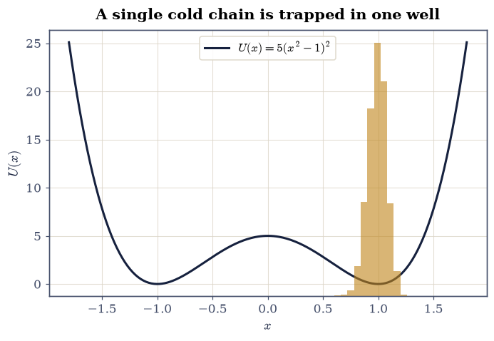
Take the symmetric double well \(U(x)=a(x^2-1)^2\) with \(a=5\), two basins at \(x=\pm1\) split by a barrier of height \(5\). At a low temperature \(T=0.25\) the Boltzmann distribution is symmetric, so a correct sampler should spend half its time in each basin. A single Metropolis chain started in the right basin does not: crossing the barrier costs \(e^{5/0.25}=e^{20}\), so it stays put for the entire run, and its sampled distribution is wrong by a factor of two.

Part a) Implement a Metropolis chain mc_chain.

Part b) Run it cold from the right basin and confirm it is trapped.

Fig. 33 The double well \(U(x)=5(x^2-1)^2\) (navy) and the distribution sampled by a single Metropolis chain at \(T=0.25\) started in the right basin (amber histogram). The chain never crosses the barrier of height 5, so it samples only the right well: a non-ergodic, and wrong, result, since the symmetric potential should populate both wells equally.

Validation 1 — the single chain is non-ergodic

Started in the right basin (\(x>0\)), the cold chain must spend essentially all its time there: a fraction near one, not the correct one-half.

✓  a single cold Metropolis chain stays trapped in one well   [fraction with x>0 = 1.000]

True

Exercise 2 — Parallel tempering escapes the barrier

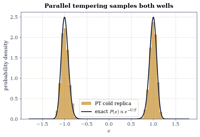
Now run several replicas at once, from a cold \(T_1=0.25\) up to a hot \(T_M=4\) where the barrier is easily crossed, and attempt swaps between adjacent temperatures with the criterion Eq. 33. A configuration that crosses the barrier in a hot replica can be swapped down to the cold one, so the cold replica, the one we care about, finally samples both wells. Because the potential is symmetric, the exact Boltzmann answer is one-half in each, and parallel tempering recovers it.

Part a) Implement parallel_tempering, returning the cold replica’s samples. Part b) Confirm the cold replica now populates both wells equally.

Fig. 34 Distribution of the cold (\(T=0.25\)) replica under parallel tempering across eight temperatures from 0.25 to 4 (amber), against the exact Boltzmann distribution \(P(x)\propto e^{-U(x)/T}\) (navy). The swaps carry barrier crossings down from the hot replicas, so the cold replica now samples both wells with the correct equal weight: the non-ergodicity of Exercise 1 is cured.

Validation 2 — the cold replica now samples both wells equally

With the swaps in place, the cold replica must populate the two symmetric wells with equal weight, the exact Boltzmann result: a fraction near one-half.

✓  parallel tempering recovers the exact symmetric Boltzmann populations   [got 0.4975 vs expected 0.5 (rtol=1e-06, atol=0.12)]

True

Part c) The swap rule Eq. 33 only accepts when the two replicas’ energies are comparable, so parallel tempering works exactly when adjacent rungs overlap in energy. Measure that overlap directly: histogram each rung’s energies on a common grid and integrate the pointwise minimum of adjacent pairs, which is the standard overlap coefficient and equals 1 for identical distributions and 0 for disjoint ones. Report the acceptance rate alongside it — the two numbers are the same statement seen from opposite sides.

Part d) Track where each configuration goes. Rewrite the sampler as pt_traced, carrying an integer label array alongside the positions and swapping labels whenever configurations swap, so the rung occupied by each original replica can be reconstructed. A configuration that starts cold should climb the ladder, cross the barrier while hot, and come back down: those round trips are the real efficiency measure of parallel tempering, far more informative than the acceptance rate alone. Write this one yourself — the implementation is the lesson.

swap acceptance = 0.863
adjacent energy overlap: min 0.872, mean 0.908
round trips of the initially-cold replica = 25
replicas visiting BOTH ends of the ladder = 8/8

Once Loop Reflect

Fig. 35 Animation of an eight-replica parallel-tempering run on the double well \(U(x)=a(x^2-1)^2\). Left: one copy of the potential per ladder rung, offset vertically so the eight configurations do not overlap, coldest at the bottom and hottest at the top (navy to yellow); height therefore encodes temperature, and the hot replicas are visibly the ones crossing the barrier while the cold ones stay pinned in a single well. Right: the rung occupied by the configuration that started coldest, over a scrolling window of Monte Carlo steps. It climbs to the hot end, crosses, and descends again — one such excursion is a round trip, and it is round trips, not swap acceptance, that measure how well the method is working.

Validation 2b — the ladder actually mixes

Three checks on the animated run, none of them on the player. Adjacent rungs must overlap in energy, since Eq. 33 cannot accept otherwise; every replica must reach both ends of the ladder, which is the definition of a mixing ladder; and the initially-cold configuration must complete round trips. The last is the sharpest: a ladder can post a high acceptance rate while configurations merely rattle between neighbouring rungs and never traverse it.

✓  adjacent rungs overlap in energy, which is the precondition eq-swap needs before it can accept anything   [min overlap 0.87, mean 0.91, swap acceptance 0.86]
✓  and every replica visits both the coldest and the hottest rung: the ladder mixes rather than merely jiggling   [8 of 8 replicas reached both ends]
✓  the initially-cold configuration completes round trips, the efficiency measure a bare acceptance rate cannot supply   [25 round trips in 2500 steps]

True

Exercise 3 — The real run: LAMMPS parallel tempering of an argon cluster

The course applied exactly this algorithm to a 38-atom argon cluster in LAMMPS, with twelve replicas. The temperatures are spread geometrically from 2 K to 40 K, a harmonic wall confines the cluster so atoms cannot evaporate at the hot end, and an exchange is attempted every 1000 steps:

variable t world  2.00 2.60 3.64 5 6.63 9.12 12.07 16 21.97 26.83 32.76 40.00
pair_style lj/cut 8.5
pair_coeff 1 1 0.01042 3.405 8.5      # argon: epsilon = 0.01042 eV, sigma = 3.405 A
fix 1 all nvt temp $t $t 0.1          # a different target temperature per replica
fix 2 all wall/region rs harmonic 2.0 0.0 0.4   # spherical confinement
temper 5000000 1000 $t 1 3678 3490    # attempt an exchange every 1000 MD steps

The full script ships with this notebook: replica-exchange.lammps. Postprocessing the output is the crux. Each processor holds a configuration whose temperature changes as swaps are accepted, so to recover the canonical average at a fixed temperature we pool every processor’s potential energy by the reference temperature it occupied at that step, read from the exchange log. We map the swaps here, and turn them into the caloric curve in Exercise 4.

The committed output ships with this notebook: the swap log swap.log records which of the twelve temperatures each replica occupies over time, and the twelve per-replica thermo logs replica_00.log … replica_11.log hold each one’s potential energy.

Part a) Read the swap log and plot the temperature index versus step for a few replicas (Assignment 1).

Part b) Confirm a replica random-walks across the whole temperature ladder, the condition for parallel tempering to help.

Fig. 36 Temperature random-walk from the real LAMMPS run: the temperature index occupied by three of the twelve replicas over the five-million-step simulation. Accepted swaps carry each replica up and down a broad span of the ladder (one reaches the cold 2 K end, another the hot 40 K end), so configurations mix across temperatures instead of staying pinned to one. This wandering, not a fixed temperature per replica, is what makes the method work.

swap activity: 32.3% of steps change a replica's temperature; a tracked replica visits 5–10 of the 12 temperatures

Validation 3 — the replicas mix across temperatures

Parallel tempering only helps if configurations actually move through temperature space. Every replica must visit a broad span of the ladder, not stay pinned at one temperature.

✓  every replica random-walks across a broad span of the temperature ladder   [replicas visit 5–10 of 12 temperatures; swaps active on 32.3% of steps]

True

Exercise 4 — The caloric curve and the melting step

Plot the energy against temperature. Below melting the cluster is a rigid solid, and its energy rises only gently as the atoms vibrate a little harder. Through the melting range the structure breaks up, and the energy jumps as the latent heat goes into disordering the cluster. That steep step, here around \(T^\ast\approx0.16\) (\(T\approx19\,\)K), is the thermodynamic signature of melting, visible directly in the caloric curve.

Part a) Plot \(\langle E\rangle\) against \(T^\ast\).

Part b) Identify the steep (melting) section and confirm it lies in the expected range for a 38-atom Lennard-Jones cluster, \(T^\ast\sim0.1\)–\(0.2\).

Fig. 37 Caloric curve of the 38-atom argon cluster from the real LAMMPS parallel-tempering run: average potential energy (eV) versus reduced temperature \(T^\ast=T/120.9\). The energy rises gently while the cluster is solid, then steeply through the melting range near \(T^\ast\approx0.16\) (amber band) as latent heat disorders the structure, then continues to climb in the liquid.

Validation 4 — melting sits where it should

The steepest rise of the caloric curve, the melting transition, must fall in the known melting range of a 38-atom Lennard-Jones cluster, \(T^\ast\approx0.1\)–\(0.2\).

✓  the caloric curve's steepest rise locates cluster melting near T* ~ 0.16   [steepest dE/dT at T* = 0.157 (T = 19 K)]

True

Exercise 5 — The heat-capacity peak

The heat capacity \(C_v=d\langle E\rangle/dT\) Eq. 34 turns the melting step into a peak. For a macroscopic system the peak would be a sharp divergence at a first-order transition; for a 38-atom cluster it is a finite, rounded bump, but it still marks the melting temperature unambiguously. This is the result the course was built around: a thermodynamic transition measured by parallel tempering.

Part a) Compute \(C_v\) from the caloric curve.

Part b) Confirm its peak coincides with the melting transition of Exercise 4.

Fig. 38 Heat capacity \(C_v=d\langle E\rangle/dT\) of the 38-atom argon cluster (in units of \(k_B\)), from the caloric curve of the real parallel-tempering run. The peak at \(T^\ast\approx0.16\) (\(T\approx19\,\)K, amber line) is the rounded, finite-size remnant of the melting transition: the cluster’s melting point, read from its heat capacity.

Validation 5 — the heat-capacity peak is a genuine melting transition

The melting feature must be a real peak: the heat capacity rises to it and falls away on the high-temperature side, the finite-size signature of the solid melting, not a monotonic ramp.

✓  C_v has a local melting peak at the caloric-curve step   [C_v/k_B at T* = 0.16: 72.5 < 149.4 > 102.3]

True

Exercise 6 — Every histogram at once: multi-histogram reweighting

Exercise 4 used the committed run twelve points at a time: one mean energy per temperature, and a finite difference for \(C_v\). But each replica’s energy histogram carries vastly more than its mean, and the histograms overlap — the very property that made the swaps work. Ferrenberg–Swendsen multi-histogram reweighting [FS89] (WHAM) combines all of them into the one object they jointly determine, the density of states \(\Omega(E)\), by solving

(35)\[\Omega(E) \;=\; \frac{\sum_r H_r(E)} {\sum_r n_r\, e^{\,f_r - \beta_r E}}, \qquad e^{-f_r} \;=\; \sum_E \Omega(E)\, e^{-\beta_r E},\]

self-consistently: the \(f_r\) are the replicas’ free energies, and each equation feeds the other until the pair stops moving. With \(\Omega(E)\) in hand, every equilibrium average at any temperature in the sampled range is a weighted sum — \(\langle E\rangle(T)\) and \(C_v(T)\) become continuous curves, and the fluctuation formula for \(C_v\), too noisy per replica in Exercise 5’s data, becomes usable because every sample in the run now contributes.

One implementation fact decides success outright: at \(T = 2\,\)K, \(\beta E \sim 10^4\), so Eq. 35 must be iterated entirely in log space (logsumexp) — the literal formula overflows on the first step.

Part a) Implement the WHAM iteration in log space and run it to self-consistency on the twelve temperature-sorted energy histograms of Exercise 4. Write this one yourself — the implementation is the lesson.

Part b) Validate the machinery: the reweighted \(\langle E\rangle(T)\) must reproduce the twelve directly measured means, and \(\ln\Omega\) must increase with \(E\) over the well-sampled range, as a density of states of a bound system in this energy window must.

Part c) Read the continuous \(C_v(T)\) — and find what the twelve-point finite difference could not show. The melting peak stands where Exercise 5 put it; below it, the curve rises again into a second, sharper feature at the coldest temperatures. Trace it to its origin in the raw data: the coldest replicas oscillate between two solid basins some \(18\,\)meV apart, occupying the deeper one about a quarter of the time at \(2\,\)K and abandoning it by \(4\,\)K. State the honest caveat: the coldest replicas equilibrate slowest, so the feature’s height is the least certain number in this notebook — but its existence is a property of the committed samples, and no finite difference across two points could ever have resolved it.

WHAM: 4196 iterations to residual 0.0e+00

Fig. 39 Multi-histogram reweighting of the committed twelve-replica run. Left: the continuous mean energy from the WHAM density of states (navy) through the twelve directly measured means (amber points) — the same data Exercise 4 used, now interpolated by physics rather than by eye, agreeing with every point to a couple of meV. Right: the continuous heat capacity, with the melting peak standing where Exercise 5’s finite difference located it, and a second, sharper low-temperature feature the finite difference could not resolve: the coldest replicas oscillate between two solid basins ~18 meV apart, and reweighting turns that two-level fluctuation into a heat-capacity signature. The height of that cold feature is the least-equilibrated number in the notebook, and the caption says so.

<E>(T) reproduces the 12 measured means to 1.94 meV (curve span 351 meV)
melting peak at 19.9 K (Ex. 5: 19.0 K); cold feature 380 kB vs trough 59 kB
deep-basin occupancy: 23.7% at 2 K -> 0.10% at 4 K

Validation 6 — the curve earns the twelve points, then exceeds them

Five checks. The iteration must reach self-consistency to machine precision. The reweighted mean energy must reproduce every directly measured mean — the new machinery earning the old data. \(\ln\Omega\) must increase over the well-sampled range, as a density of states here must. The melting peak must stand where Exercise 5’s finite difference put it. And the cold feature must be a genuine two-basin property of the committed samples: a substantial deep-basin occupancy at the coldest rung that has collapsed two rungs up.

✓  the WHAM equations reached self-consistency to machine precision, in log space -- the literal form of eq-wham overflows at these temperatures   [residual 0.0e+00 after 4196 iterations]
✓  the reweighted mean energy reproduces all twelve directly measured means to a few meV: the density of states earns the data it came from   [max deviation 1.94 meV over a 351 meV span]
✓  ln Omega increases with E across the well-sampled range, as the density of states of a bound cluster below its dissociation must   [monotone over 49 well-sampled bins]
✓  the continuous heat capacity puts the melting peak where the finite difference of Exercise 5 put it -- same physics, sharper instrument   [got 19.8958 vs expected 18.985 (rtol=0.15, atol=1e-09)]
✓  and the low-temperature feature the finite difference could not resolve is a genuine two-basin oscillation of the committed samples: substantial deep-basin occupancy at the coldest rung, gone two rungs up the ladder   [cold feature 380 kB vs trough 59 kB; deep occupancy 23.7% -> 0.10%]

True

Notebook summary

We saw why a single cold chain is trapped, then watched parallel tempering cure it: swapping configurations up and down a temperature ladder let the cold replica sample both wells with the correct Boltzmann weight. Applied to the course’s real twelve-replica LAMMPS run, the swap log showed each replica random-walking across the ladder, and pooling each replica’s potential energy by the temperature it occupied reconstructed the caloric curve. Its steepest rise, a peak in the heat capacity near \(T^\ast\approx0.16\) (\(\approx19\,\)K), located the melting transition of the 38-atom cluster.

The deepening then spent the same data all at once: Ferrenberg–Swendsen reweighting, iterated in log space to machine self-consistency, turned the twelve histograms into a density of states that reproduces every measured mean to two meV and renders \(C_v(T)\) continuous — the melting peak standing where the finite difference put it, plus a sharp cold feature no finite difference could resolve: the coldest replicas’ own two-basin oscillation, occupying a deeper solid basin a quarter of the time at 2 K and abandoning it by 4 K.

Outlook

• Better heat capacities. The committed run is short, so \(C_v\) from energy fluctuations, \(C_v=(\langle E^2\rangle-\langle E\rangle^2)/(k_BT^2)\), is noisy here; the multiple-histogram (WHAM) method combines all temperatures to sharpen both the caloric curve and the peak.

• The solid-solid transition. Below melting the 38-atom cluster also converts between its truncated-octahedron and icosahedron forms (Volume II); a finer temperature grid resolves the small low-temperature heat-capacity feature this produces.

• Order parameters. Tracking the Steinhardt \(Q_4\) or \(Q_6\) (notebook 2.1) along the replicas shows the structural change through the transition, not just its energy.

• Finding the global minimum. Because parallel tempering crosses funnels, a low replica eventually settles into the global truncated octahedron that defeated the single-funnel basin-hopping of Volume II.

References

[AT17]

Michael P. Allen and Dominic J. Tildesley. Computer Simulation of Liquids. Oxford University Press, 2 edition, 2017.

[FS89]

Alan M. Ferrenberg and Robert H. Swendsen. Optimized monte carlo data analysis. Physical Review Letters, 63(12):1195–1198, 1989. doi:10.1103/PhysRevLett.63.1195.

[FS02]

Daan Frenkel and Berend Smit. Understanding Molecular Simulation: From Algorithms to Applications. Academic Press, 2 edition, 2002.

Take this notebook with you

Use the download button (↓) in the toolbar above to save this notebook and run it yourself. The published notebooks ship without worked solutions; if you would like the reference solutions — to teach from or to check your own work — get in touch: hello@ramador.me.

Based on the lecture and exercise materials of Molecular and Materials Modelling (ETH Zürich and Empa, FS 2023), developed by Prof. Dr. Daniele Passerone (lectures), Dr. Carlo Pignedoli, and the author (exercises); here synthesised, expanded, and restyled by the author.