


1.6 Linear Maps and Change of Basis#
Notebook overview#
There is a distinction this notebook exists to draw, and it is easy to skate past: a matrix is not a linear map. A linear map is a rule taking vectors to vectors. A matrix is what that rule looks like once a basis has been chosen. Choose a different basis and the entries change completely while the map does not change at all.
The consequence is a strategy that organises the rest of the course. If a matrix is only a description, then a badly-behaved matrix might just be a badly-chosen description, and the right move is to look for a better basis. That is exactly what diagonalisation is (§3.1), what the spectral theorem promises for symmetric matrices (§3.2), and what the SVD achieves for every matrix whatsoever (§4.1) by allowing two bases instead of one.
We start concretely, in the plane, where a linear map is something you can watch: rotation, reflection, shear, scaling, projection. Each is a \(2\times2\) matrix, and their differences show up as properties of that matrix — the determinant is the area factor, orthogonality means lengths are preserved, idempotence means the map is a projection. Then we leave \(\mathbb{R}^2\): the derivative is a linear map on polynomials, so it has a \(4\times4\) matrix on \(P_3\), and that matrix is nilpotent — \(D^4 = 0\) — which is the statement that differentiating a cubic four times gives zero, wearing a matrix costume.
The notebook closes with similarity. The same derivative, written in the Legendre basis of §1.5, is a different matrix with different entries; the two are related by \(B^{-1}AB\) and share everything that belongs to the map rather than to the description — rank, trace, determinant, nilpotency, eigenvalues.
How to read a check. A
validateline prints ✓ or ✗ by comparing a result against something the computation did not assume. A ✗ flags a mismatch to investigate, never a verdict on its own.
Theory in brief#
From map to matrix#
A map \(T : V \to W\) is linear when \(T(\alpha u + \beta v) = \alpha T(u) + \beta T(v)\). Fix bases \(B = (b_1,\dots,b_n)\) of \(V\) and \(C\) of \(W\). Since every \(v\) is \(\sum_j c_j b_j\), linearity gives \(T(v) = \sum_j c_j\,T(b_j)\), so \(T\) is determined entirely by what it does to the basis vectors. Recording each \(T(b_j)\) in \(C\)-coordinates as a column produces the matrix
Feed the map each basis vector and write down what comes out. That is the entire construction, and it works whether the vectors are columns of numbers, polynomials, or matrices.
The five maps of the plane#
With the standard basis of \(\mathbb{R}^2\), Eq. 88 gives the familiar catalogue:
map |
matrix |
\(\det\) |
character |
|---|---|---|---|
rotation by \(\theta\) |
\(\begin{psmallmatrix}\cos\theta & -\sin\theta\\ \sin\theta & \cos\theta\end{psmallmatrix}\) |
\(+1\) |
orthogonal |
reflection in a line at \(\theta\) |
\(\begin{psmallmatrix}\cos 2\theta & \sin 2\theta\\ \sin 2\theta & -\cos 2\theta\end{psmallmatrix}\) |
\(-1\) |
orthogonal, symmetric |
shear by \(k\) |
\(\begin{psmallmatrix}1 & k\\ 0 & 1\end{psmallmatrix}\) |
\(+1\) |
area-preserving, not orthogonal |
scaling by \((a,b)\) |
\(\begin{psmallmatrix}a & 0\\ 0 & b\end{psmallmatrix}\) |
\(ab\) |
diagonal |
projection onto the \(x\)-axis |
\(\begin{psmallmatrix}1 & 0\\ 0 & 0\end{psmallmatrix}\) |
\(0\) |
idempotent, singular |
The determinant is the area factor#
A linear map takes the unit square to a parallelogram, and
with the sign of \(\det A\) recording whether orientation was preserved. A singular map flattens the square onto a segment, area zero, which is the geometric meaning of \(\det A = 0\). §1.7 develops this properly; here we simply measure it.
Similarity#
Suppose \(T : V \to V\) and we change basis from \(B\) to \(B'\), with \(M\) the change-of-basis matrix of Eq. 80. Chasing Eq. 88 through gives
Two matrices related this way are similar. They describe the same map, so everything intrinsic to the map is shared: rank, trace, determinant, characteristic polynomial, eigenvalues, nilpotency. Everything else — the individual entries, the norm, the symmetry — belongs to the basis and can change freely. Recognising which is which is most of the skill.
Affine maps and homogeneous coordinates#
A translation \(\mathbf{x} \mapsto \mathbf{x} + \mathbf{t}\) is not linear: it moves the origin. The standard repair is to work one dimension up, writing a point \((x, y)\) as \((x, y, 1)\) and using
Now every affine transformation is a single matrix, compositions are products, and a whole graphics pipeline is one chain of multiplications. This is why every graphics API works in \(4\times4\) matrices for three-dimensional scenes.
Setup#
import numpy as np
import sympy as sp
import matplotlib.pyplot as plt
from matplotlib.animation import FuncAnimation

from ecp import animate, validate
from ecp import linalg as la
from ecp.style import use_style

use_style()
rng = np.random.default_rng(0)  # every random object below comes from this seed

xs = sp.symbols("x")
np.set_printoptions(precision=5, suppress=True, linewidth=110)

THETA = np.pi / 6  # the rotation and reflection angle used throughout


def rotation(theta):
    """Matrix of the rotation by ``theta`` about the origin, in the standard basis."""
    c, s = np.cos(theta), np.sin(theta)
    return np.array([[c, -s], [s, c]])


def reflection(theta):
    """Matrix of the reflection in the line through the origin at angle ``theta``."""
    c, s = np.cos(2 * theta), np.sin(2 * theta)
    return np.array([[c, s], [s, -c]])


MAPS = {
    "rotation": rotation(THETA),
    "reflection": reflection(THETA),
    "shear": np.array([[1.0, 0.8], [0.0, 1.0]]),
    "scaling": np.array([[2.0, 0.0], [0.0, 1.5]]),
    "projection": np.array([[1.0, 0.0], [0.0, 0.0]]),
}

UNIT_SQUARE = np.array([[0.0, 0.0], [1.0, 0.0], [1.0, 1.0], [0.0, 1.0]])


def shoelace_area(pts):
    """Area of a simple polygon from its vertices, by the shoelace formula.

    Measures the area of the image of the unit square directly from its corners,
    without reference to any determinant. That independence is what makes it a
    real check of Eq. 3 rather than a restatement of it: the two quantities are
    computed by completely different routes and required to agree.

    Parameters
    ----------
    pts : numpy.ndarray, shape (k, 2)
        Polygon vertices in order, without repeating the first.

    Returns
    -------
    float
        The enclosed area, always non-negative.
    """
    x, y = pts[:, 0], pts[:, 1]
    return 0.5 * abs(float(np.dot(x, np.roll(y, -1)) - np.dot(y, np.roll(x, -1))))
Exercise 1 — Five maps, and what their matrices reveal#
Each of the five maps in the theory table does something visibly different to the plane, and each difference corresponds to an algebraic property of the matrix. This exercise draws all five and reads the properties off.
The correspondences to establish, with \(\theta = \pi/6\), shear \(k = 0.8\), and scaling \((2, 1.5)\):
Rotation and reflection are orthogonal (\(M^{\top}M = I\)), so they preserve every length and angle. Their determinants are \(+1\) and \(-1\), the sign recording whether the plane is flipped over.
The shear preserves area but not length: \(\det = 1\) yet \(M^{\top}M \neq I\). Horizontal lines slide over one another.
The scaling is diagonal, so the axes are its invariant directions — already a preview of eigenvectors.
The projection is idempotent (\(P^2 = P\)) and singular (\(\det = 0\)): applying it twice does nothing new, and it destroys a whole dimension.
Part a) Build the five matrices with the rotation, reflection helpers
and explicit arrays, and verify linearity numerically for each: over 200 random
pairs \(\mathbf{u}, \mathbf{v}\) and scalars \(\alpha, \beta\) from
rng.standard_normal, check
\(M(\alpha\mathbf{u} + \beta\mathbf{v}) = \alpha M\mathbf{u} + \beta M\mathbf{v}\)
to \(10^{-13}\).
Part b) For each, report \(\det M\), whether \(M^{\top}M = I\), whether \(M^2 = M\), and whether \(M = M^{\top}\), and confirm the classifications above.
Part c) Draw all five with ecp.linalg.grid_transform, showing a reference
lattice and its image, so the geometric character of each is visible beside its
algebra.
map                det  orthogonal  idempotent  symmetric   linearity
rotation       +1.0000        True       False      False    8.88e-16
reflection     -1.0000        True       False       True    8.88e-16
shear          +1.0000       False       False      False    8.88e-16
scaling        +3.0000       False       False       True    8.88e-16
projection     +0.0000       False        True       True    0.00e+00
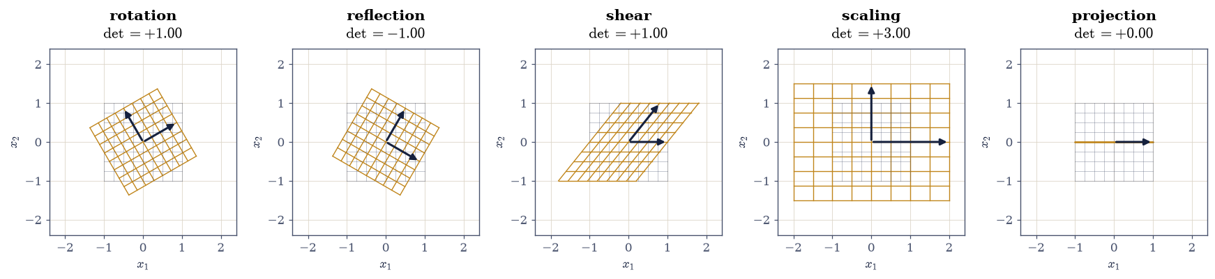
Fig. 34 The five linear maps of the plane acting on a reference lattice: a faint grey grid is the domain and the amber grid its image, with the two ink arrows showing where the standard basis vectors \(\mathbf{e}_1\) and \(\mathbf{e}_2\) land. Rotation and reflection preserve every length; the shear slides horizontal lines over one another while preserving area; the scaling stretches along the axes, which are its invariant directions; and the projection collapses the whole plane onto a line, which is what \(\det = 0\) means geometrically.#
Validation 1#
Linearity is checked over a sample rather than asserted, and each structural property is checked against the classification the theory table predicted, so the table is verified rather than illustrated.
✓  all five maps are linear, over 200 random combinations each   [largest defect 8.9e-16]
✓  rotation and reflection are orthogonal; the shear is not   [orthogonality is exactly preservation of every length and angle]
✓  the five determinants are +1, -1, +1, +3, 0   [max|Δ| = 4.44089e-16 (rtol=0, atol=1e-12)]
✓  the projection is idempotent (P^2 = P) and the rotation is not   [applying a projection twice does nothing new]
✓  the reflection is symmetric while the rotation is not   [a reflection is its own inverse; a rotation's inverse is the opposite turn]
True
Exercise 2 — The determinant is the area factor#
Eq. 89 claims a geometric meaning for a quantity we have so far
only computed. The claim is checkable, and the check is worth doing carefully
because the two sides are computed by completely unrelated routes: one from the
matrix entries by np.linalg.det, one from the corners of the image polygon
by the shoelace formula, which never sees the matrix at all.
Applying each map to the unit square with corners \((0,0), (1,0), (1,1), (0,1)\) gives a parallelogram, and its area should equal \(|\det M|\): exactly 1 for the rotation, reflection and shear, exactly 3 for the scaling by \((2, 1.5)\), and exactly 0 for the projection, which flattens the square onto a segment.
The animation makes the continuity visible. Interpolating linearly from the identity to a target matrix, \(M(t) = (1-t)I + tM\), deforms the grid smoothly, and the area sweeps continuously from 1 to \(|\det M|\) — passing through zero if the family crosses a singular matrix, which is the moment the plane collapses.
Part a) Map the unit square by each of the five matrices and measure the
image area with the shoelace_area helper, comparing against \(|\det M|\) to
\(10^{-12}\).
Part b) Confirm the sign story: compute the signed shoelace area (drop the absolute value) and confirm it is negative exactly for the reflection, which is the map that turns the plane over.
Part c) Animate the interpolation \(M(t) = (1-t)I + tM_{\text{shear-rotate}}\) for \(t \in [0,1]\), where \(M_{\text{shear-rotate}}\) is the rotation by \(\pi/6\) composed with the shear, showing the grid deforming and the area evolving.
map           measured area    |det M|         gap     signed
rotation        1.000000000   1.000000    0.00e+00    +1.0000
reflection      1.000000000   1.000000    0.00e+00    -1.0000
shear           1.000000000   1.000000    1.11e-16    +1.0000
scaling         3.000000000   3.000000    4.44e-16    +3.0000
projection      0.000000000   0.000000    0.00e+00    +0.0000
Fig. 35 Animation of the linear interpolation \(M(t) = (1-t)I + tM\) from the identity to the composition of a shear with a rotation by \(\pi/6\), acting on a reference lattice. The grid deforms continuously because the family of matrices does, and the signed area of the image of the unit square, printed in the corner, sweeps continuously from 1 to \(\det M\) — the determinant is a continuous function of the entries, and it measures area at every instant, not only at the endpoints.#
Validation 2#
The area identity is checked against a measurement that never touches the matrix, which is what makes it evidence for Eq. 89 rather than a tautology. The animation’s validation checks the data it displays — the area at every frame against \(\det M(t)\) — never the animation object, since there are many valid ways to build one.
✓  the measured image area equals |det M| for all five maps (Eq. 3)   [max|Δ| = 4.44089e-16 (rtol=0, atol=1e-12)]
✓  and the signed area is negative exactly for the reflection   [the sign of the determinant records whether the plane was turned over]
✓  the projection flattens the square to zero area, matching det = 0   [got 0 vs expected 0 (rtol=0, atol=1e-14)]
✓  and at EVERY animated frame the area equals det M(t)   [max|Δ| = 2.22045e-16 (rtol=0, atol=1e-12)]
True
Exercise 3 — The derivative is a matrix#
Now the payoff of §1.5. Differentiation takes polynomials to polynomials and satisfies \((\alpha p + \beta q)' = \alpha p' + \beta q'\), so it is a linear map on \(P_3\) — and therefore, by Eq. 88, it has a \(4\times4\) matrix.
Building it is the recipe: differentiate each basis vector and record the result in coordinates. With the monomial basis \((1, x, x^2, x^3)\), the derivatives are \(0, 1, 2x, 3x^2\), whose coordinate columns give
Everything about differentiation on \(P_3\) is now visible in the matrix. \(D\) is strictly upper triangular, so it is nilpotent: \(D^4 = 0\) but \(D^3 \neq 0\), which says that differentiating a cubic four times gives zero and three times does not. Its rank is 3, so its null space is one-dimensional — the constants, the functions with zero derivative. And its diagonal is entirely zero, so its only eigenvalue is 0 with multiplicity 4, which is why §3.5 calls such matrices defective: there are nowhere near enough eigenvectors to build a basis.
Integration is the near-inverse. It maps \(P_3 \to P_4\), so it is not square, but restricted to the polynomials with zero constant term it undoes \(D\) exactly — which is the fundamental theorem of calculus expressed as a statement about one-sided inverses.
Part a) Build \(D\) from Eq. 92 by differentiating each
monomial with sympy.diff and extracting coordinates, and confirm it matches
the stated matrix exactly.
Part b) Confirm the structural facts: \(D^4 = 0\) and \(D^3 \neq 0\) exactly, \(\operatorname{rank} D = 3\), and the null space is spanned by the constant polynomial 1.
Part c) Confirm \(D\) agrees with actual differentiation: for 50 random cubics with integer coefficients, check that applying \(D\) to the coordinate column gives the coordinates of the symbolic derivative, exactly.
D, the derivative on P_3 in the monomial basis:
⎡0  1  0  0⎤
⎢          ⎥
⎢0  0  2  0⎥
⎢          ⎥
⎢0  0  0  3⎥
⎢          ⎥
⎣0  0  0  0⎦

matches Eq. 5 exactly : True
D^3 = 0               : False
D^4 = 0               : True
rank D                : 3
null space            : [[1, 0, 0, 0]]   (the constants)
eigenvalues           : {0: 4}
D applied to coordinates == coordinates of the derivative, over 50 random cubics: True
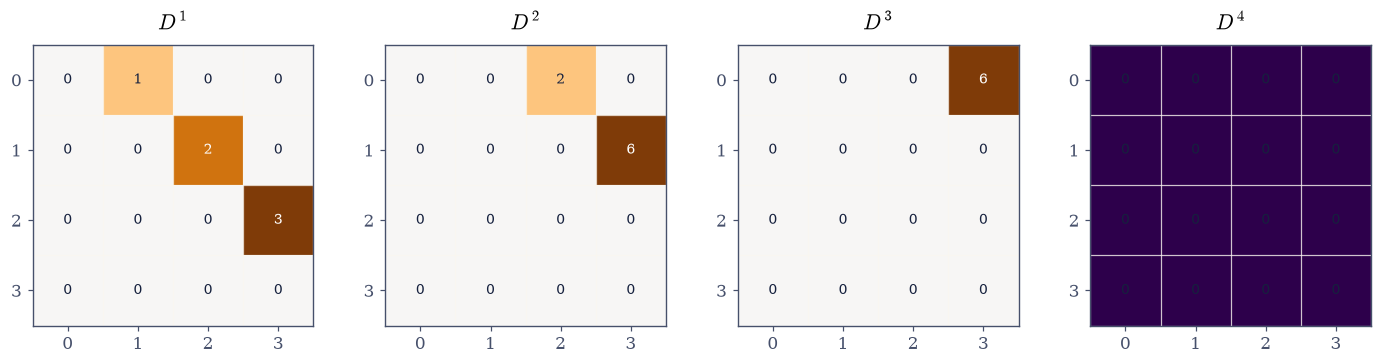
Fig. 36 The derivative on \(P_3\) as a matrix in the monomial basis (Eq. 5) and its powers, on a diverging colour scale centred at zero. The single superdiagonal \(1, 2, 3\) moves one place further from the diagonal at each power, so \(D^4\) is identically zero: the matrix is nilpotent, which is the statement that differentiating a cubic four times gives zero, written as an algebraic property.#
Validation 3#
Every check is exact rational arithmetic. The last one is the important one: it
verifies that the matrix genuinely is differentiation, by comparing its
action on coordinate columns against sympy.diff on the polynomials
themselves — two routes that share no code.
✓  the derivative matrix on P_3 is exactly the D of Eq. 5   [built by differentiating each basis vector and taking coordinates]
✓  D is nilpotent of index exactly 4: D^4 = 0 but D^3 != 0   [differentiate a cubic four times and it vanishes; three does not]
✓  rank D = 3 with a one-dimensional null space   [the null space is the constants, the polynomials with zero derivative]
✓  its only eigenvalue is 0, with algebraic multiplicity 4   [a defective matrix: far too few eigenvectors to form a basis]
✓  and D really is differentiation, checked against sympy.diff   [over 50 random cubics, exactly]
True
Exercise 4 — The same map, two matrices#
Here is the notebook’s thesis, made concrete. Write the same derivative in the Legendre basis \((P_0, P_1, P_2, P_3)\) of §1.5 and a different matrix appears:
with \(M\) the change-of-basis matrix of §1.5 Eq. 85. Different entries, different superdiagonal, an extra nonzero in the corner. Same map.
What is shared is precisely what belongs to the map: rank 3, trace 0, determinant 0, the single eigenvalue 0 with multiplicity 4, and nilpotency of index exactly 4. What differs — the individual entries, and for instance the Frobenius norm, which is \(\sqrt{14}\) against \(\sqrt{36}\) — belongs to the description. Sorting quantities into those two boxes is the skill this notebook exists to build, and it is what makes Volume III possible: if a property is basis-independent, you may hunt for a basis that displays it clearly.
Part a) Build \(M\) (Legendre polynomials in monomial coordinates), form \(D_L = M^{-1}DM\) exactly, and confirm it matches Eq. 93.
Part b) Verify \(D_L\) independently: build it directly from Eq. 88 by differentiating each Legendre polynomial and taking Legendre coordinates, and confirm the two constructions agree exactly.
Part c) Tabulate what is preserved and what is not: rank, trace, determinant, eigenvalues, nilpotency index (preserved), against the entries and the Frobenius norm (not).
M (Legendre in monomial coordinates):
⎡1  0  -1/2   0  ⎤
⎢                ⎥
⎢0  1   0    -3/2⎥
⎢                ⎥
⎢0  0  3/2    0  ⎥
⎢                ⎥
⎣0  0   0    5/2 ⎦

D_L = M^-1 D M:
⎡0  1  0  1⎤
⎢          ⎥
⎢0  0  3  0⎥
⎢          ⎥
⎢0  0  0  5⎥
⎢          ⎥
⎣0  0  0  0⎦

matches Eq. 6 exactly            : True
agrees with the direct construction: True

quantity                     monomial D     Legendre D_L   same?
rank                                  3                3    True
trace                                 0                0    True
determinant                           0                0    True
eigenvalues                      {0: 4}           {0: 4}    True
nilpotency index                      4                4    True
Frobenius norm                   3.7417           6.0000   False
entry (0, 3)                          0                1   False
Validation 4#
The two constructions of \(D_L\) — one by similarity from \(D\), one built directly from the Legendre basis — share no code and must agree exactly. The invariants are checked to be equal and the non-invariants to be different, which is what makes the distinction between them real rather than rhetorical.
✓  the derivative in the Legendre basis is exactly the D_L of Eq. 6   [computed by similarity, M^-1 D M]
✓  and the direct construction from Eq. 2 gives the same matrix exactly   [two routes sharing no code: similarity, and differentiating the basis]
✓  rank, trace, determinant and eigenvalues are all preserved by similarity   [these belong to the map, not to the basis it is written in]
✓  so is nilpotency of index exactly 4   [the same map, however it is written]
✓  while the entries and the Frobenius norm differ: those belong to the basis   [||D||_F = 3.7417 against ||D_L||_F = 6.0000]
True
Exercise 5 — Composition, and why order is geometric#
Eq. 40 in §1.1 defined the product so that it represents composition. In the plane that becomes visible: rotating then shearing does something different from shearing then rotating, and you can see which is which.
The determinant, by contrast, does not notice: \(\det(AB) = \det A \det B\) is symmetric in \(A\) and \(B\), so both orders change area by the same factor. Order affects the shape of the image, not its size. That is a useful reminder that the determinant, for all its geometric meaning, throws a great deal away.
Part a) For \(R\) the rotation by \(\pi/6\) and \(S\) the shear by \(0.8\), compute \(RS\) and \(SR\), confirm they differ, and report the commutator \(RS - SR\) and its Frobenius norm relative to \(\|R\|_F\|S\|_F\).
Part b) Confirm both have the same determinant, and that both equal \(\det R \cdot \det S = 1\).
Part c) Draw the unit square under \(R\), \(S\), \(RS\) and \(SR\) on one figure so the difference in shape is visible while the areas are equal.
RS =
 [[0.86603 0.19282]
 [0.5     1.26603]]
SR =
 [[1.26603 0.19282]
 [0.5     0.86603]]

RS - SR =
[[-0.4  0. ]
 [ 0.   0.4]]
relative commutator norm  : 0.246183
det(RS) = 1.0000000000   det(SR) = 1.0000000000
det R * det S = 1.0000000000
areas equal: 0.00e+00
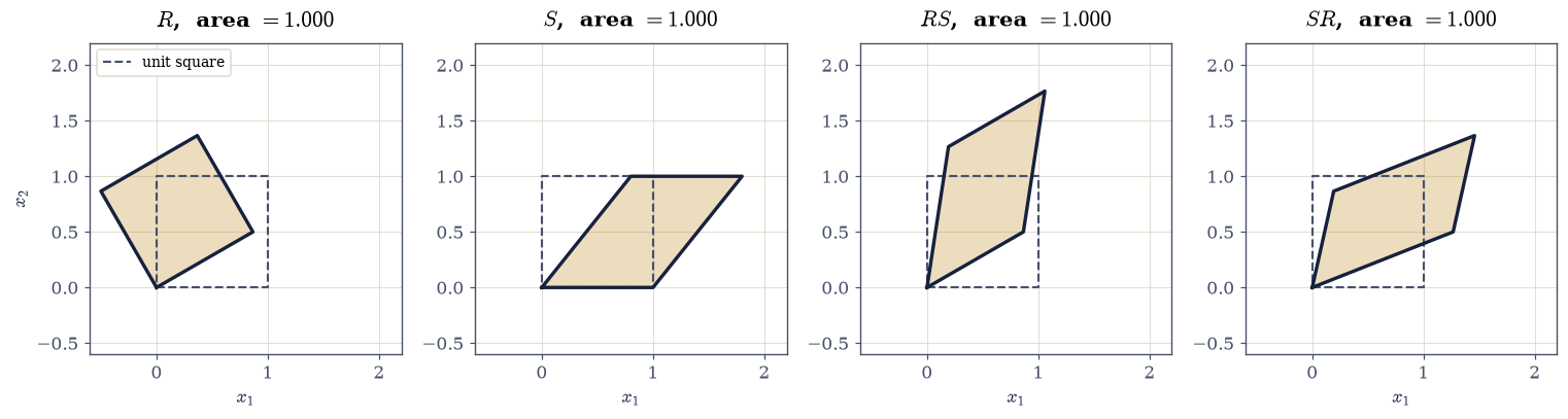
Fig. 37 The unit square (grey) under the rotation \(R\) by \(\pi/6\), the shear \(S\) by \(0.8\), and the two compositions \(RS\) (rotate first, then shear) and \(SR\) (shear first, then rotate). The two composite images are different quadrilaterals, because composition does not commute, yet both enclose exactly the same area, because \(\det(RS) = \det(SR) = \det R \cdot \det S\) regardless of order.#
Validation 5#
Non-commutativity is checked as a genuine difference rather than a small one, and the equality of determinants is checked despite it — the two facts together are the content of the exercise.
✓  RS and SR are genuinely different: composition does not commute   [relative commutator norm 0.2462]
✓  yet their determinants are equal, since det(AB) = det A det B is symmetric   [got 1 vs expected 1 (rtol=0, atol=1e-14)]
✓  and both equal det R times det S   [got 1 vs expected 1 (rtol=0, atol=1e-14)]
✓  so the two images enclose the same area despite being different shapes   [got 1 vs expected 1 (rtol=0, atol=1e-14)]
True
Exercise 6 — Affine maps, and the trick of going up a dimension#
Translation breaks linearity: \(T(\mathbf{x}) = \mathbf{x} + \mathbf{t}\) sends \(\mathbf{0}\) to \(\mathbf{t}\), and a linear map must fix the origin. Since translation is unavoidable in any real application, the standard repair is Eq. 91: embed the plane as the slice \(z = 1\) of \(\mathbb{R}^3\), where translation becomes a shear and is therefore linear after all.
The payoff is compositional. Rotating about an arbitrary point \(\mathbf{c}\) — not the origin — is “translate by \(-\mathbf{c}\), rotate, translate back”, which as homogeneous matrices is a single product \(T_{\mathbf{c}} R T_{-\mathbf{c}}\). Chaining an entire scene transformation into one matrix is why every graphics pipeline in existence works this way.
Part a) Build the homogeneous matrices for a translation by \(\mathbf{t} = (2, -1)^{\top}\) and a rotation by \(\pi/3\), apply each to the point \((1, 0)\) written as \((1, 0, 1)\), and confirm the results are \((3, -1)\) and \((\tfrac12, \tfrac{\sqrt3}{2})\) to \(10^{-14}\).
Part b) Confirm translation is genuinely not linear in the plane: show \(T(\mathbf{0}) \neq \mathbf{0}\) and \(T(2\mathbf{x}) \neq 2T(\mathbf{x})\) for \(\mathbf{x} = (1,1)^{\top}\), while the homogeneous \(3\times3\) version is linear on \(\mathbb{R}^3\).
Part c) Compose a rotation by \(\pi/2\) about the point \(\mathbf{c} = (2,1)\) as \(T_{\mathbf{c}} R T_{-\mathbf{c}}\), confirm \(\mathbf{c}\) is a fixed point of the result to \(10^{-14}\), and that the composite is not a pure rotation (its translation part is nonzero).
With your assistant
Ask for a routine that, given a list of homogeneous \(3\times3\) transformations, returns the single matrix equivalent to applying them in order, plus a function that decomposes any such matrix back into a rotation angle, a scaling, a shear and a translation. Then check it yourself: composing then decomposing must recover the inputs to \(10^{-10}\) for a random chain of five transformations, and the decomposition of a pure rotation by \(\pi/4\) must return exactly that angle with unit scaling and zero shear. The check is yours.
translate (1,0) by (2,-1) : [ 3. -1.]   expected (3, -1)
rotate (1,0) by pi/3      : [0.5     0.86603]   expected (0.5, 0.866025)

translation in the plane is not linear:
  T(0)   = [ 2. -1.]   != 0
  T(2x)  = [4. 1.]   vs  2 T(x) = [6. 0.]
  but the 3x3 homogeneous version IS linear on R^3: defect 1.78e-15

rotation by pi/2 about c = [2. 1.]:
  H c   = [2. 1.]   (c is fixed: 0.00e+00)
  translation part = [ 3. -1.]   (nonzero: not a pure rotation)
Validation 6#
The failure of linearity and the restoration of it one dimension up are checked as the same claim seen twice, which is the content of Eq. 91. The fixed-point check verifies the composition did what it was built to do, using a property the construction never referenced.
✓  the homogeneous translation moves (1,0) to (3,-1)   [max|Δ| = 0 (rtol=0, atol=1e-14)]
✓  and the homogeneous rotation by pi/3 sends it to (1/2, sqrt(3)/2)   [max|Δ| = 1.11022e-16 (rtol=0, atol=1e-14)]
✓  translation in the plane is NOT linear: it moves the origin   [which is why an extra dimension is needed at all]
✓  yet the 3x3 homogeneous matrix IS linear on R^3 (200 random combinations)   [defect 1.8e-15: the affine map became linear one dimension up]
✓  the composite fixes the point c it was built to rotate about   [max|Δ| = 0 (rtol=0, atol=1e-14)]
✓  and it is not a pure rotation: its translation part is nonzero   [translation part [ 3. -1.]]
True
Notebook summary#
A matrix is a map plus a basis. Change the basis and the entries change while the map does not.
The concrete results:
the five plane maps were confirmed linear over 200 random combinations each, with determinants exactly \(+1, -1, +1, +3, 0\); rotation and reflection came out orthogonal, the projection idempotent, the reflection symmetric and the rotation not;
the image of the unit square had area exactly \(|\det M|\) for all five, measured by the shoelace formula from the corners — a route that never touches the matrix — and the signed area was negative exactly for the reflection, the map that turns the plane over;
the animation confirmed the identity at every frame: interpolating \(M(t) = (1-t)I + tM\), the measured area tracked \(\det M(t)\) to \(10^{-12}\) across all 60 frames;
the derivative on \(P_3\) came out as the strictly-upper-triangular matrix Eq. 92 with \(D^4 = 0\) and \(D^3 \neq 0\) exactly, rank 3, null space the constants, and eigenvalue \(0\) with multiplicity 4 — and it was verified to be differentiation by checking against
sympy.diffon 50 random cubics;the same derivative in the Legendre basis was a different matrix, Eq. 93, obtained two independent ways that agreed exactly, sharing rank, trace, determinant, eigenvalues and nilpotency index with \(D\) while differing in its entries and in Frobenius norm (\(\sqrt{14}\) against \(\sqrt{36}\));
composition did not commute (relative commutator norm \(0.246\)) yet both orders gave identical determinants and identical areas;
and translation, not linear in the plane, became linear one dimension up, with the composite \(T_{\mathbf{c}}RT_{-\mathbf{c}}\) fixing \(\mathbf{c}\) to \(10^{-14}\).
Methods met: Eq. 88 as a recipe (feed the map each basis
vector), the shoelace formula as an independent area measurement,
ecp.linalg.grid_transform, FuncAnimation with ecp.animate.show, exact
similarity \(M^{-1}DM\) in SymPy, and homogeneous coordinates.
Outlook#
Choosing the basis on purpose. Similarity lets you hunt for a basis in which a matrix is simple. The best possible case is diagonal, and §3.1 asks when that is achievable — the derivative of Exercise 3, with its single eigenvalue and too few eigenvectors, is exactly the case where it is not.
Two bases instead of one. Similarity uses the same basis on both sides, \(M^{-1}AM\). Allowing different bases for input and output gives \(U^{\top}AV\), and with that extra freedom every matrix becomes diagonal. That is the SVD, and §4.1 builds it.
The determinant, properly. Exercise 2 measured \(|\det|\) as an area without ever defining the determinant beyond
np.linalg.det. §1.7 gives the definitions, the algorithms, and the reason no numerical library computes it by cofactors.Nilpotency is not an accident. \(D^4 = 0\) on \(P_3\) generalises: any nilpotent map has a basis in which its matrix is a tidy pattern of ones on a superdiagonal, which is the Jordan form. §3.5 builds it and then explains why no numerical library will compute it for you.
References#
Sheldon Axler. Linear Algebra Done Right. Undergraduate Texts in Mathematics. Springer, 4 edition, 2024. doi:10.1007/978-3-031-41026-0.
Gilbert Strang. Introduction to Linear Algebra. Wellesley-Cambridge Press, Wellesley, MA, 6 edition, 2023. ISBN 978-1-7331466-7-8.