1.7 Determinants, Volume, and Orientation

Linear Algebra in Python

Volume I — Matrices, Elimination, and Subspaces Notebook 1.7

One number that decides invertibility, measures volume, and records orientation — computed three ways, two of which are catastrophic, and reported as zero for a matrix that is not singular.

Level · intermediate   •   Est. · 75–105 min

Raymond Amador v0.1.0  ·  2026-08-06  ·  CC BY 4.0 (text) / MIT (code)

Notebook overview

The determinant has an odd position in this course. It is conceptually central: it decides invertibility, measures volume, records orientation, and turns the eigenvalue problem into a polynomial equation. It is also, as a computational object, close to useless — no serious numerical library ever asks for it, and there is a good case that a first course should teach the theory and then advise the reader never to compute one.

This notebook makes both halves concrete. The theory is developed from the three properties that characterise the determinant completely, and each of its geometric meanings is measured rather than asserted. Then we find out what happens when a machine tries to produce the number.

What happens is worse than slowness. The definition as a sum over permutations costs \(n!\) terms, which at \(n = 8\) already takes a fifth of a second against four microseconds for the library routine — and \(n = 20\) would take longer than the age of the universe. That much is expected. The unexpected part is the range: a determinant is a product of \(n\) numbers, so it overflows and underflows with abandon. np.linalg.det of a \(260\times260\) random matrix returns inf, and — the case worth remembering — np.linalg.det of the \(60\times60\) Hilbert matrix returns exactly zero for a matrix that is perfectly nonsingular. Its determinant is about \(10^{-846}\), and float64 has no way to say so.

A reader who concluded “determinant is zero, therefore singular” would be wrong, and wrong for a reason that has nothing to do with the mathematics. The repair is slogdet, which returns the sign and the logarithm separately and never leaves the representable range. And the deeper repair is the one §1.3 already gave: singularity is a question about singular values, not about determinants.

How to read a check. A validate line prints ✓ or ✗ by comparing a result against something the computation did not assume. A ✗ flags a mismatch to investigate, never a verdict on its own.

Scope. Axler [Axl24] famously postpones determinants to the final chapter and derives the spectral theory without them, which is worth knowing as a counterweight; Strang [Str23] Chapter 5 gives the classical development this notebook follows.

Theory in brief

Three properties that pin it down

The determinant of an \(n\times n\) matrix is the unique function of its rows satisfying three conditions:

1. Multilinearity. It is linear in each row separately, the others held fixed.

2. Alternation. Swapping two rows flips the sign — equivalently, a matrix with two equal rows has determinant zero.

3. Normalisation. \(\det I = 1\).

Everything else follows. From these, the value on any matrix is forced, and carrying the argument through gives the explicit formula

(94)\[\det A = \sum_{\sigma \in S_n} \operatorname{sgn}(\sigma) \prod_{i=1}^{n} a_{i,\sigma(i)} ,\]

a sum over all \(n!\) permutations. That is a definition, not an algorithm: at \(n = 20\) there are \(2.4\times10^{18}\) terms.

How it is actually computed

Elimination already produces it. From \(PA = LU\) of §1.2, taking determinants and using \(\det L = 1\) (unit diagonal) and \(\det P = \pm1\) gives

(95)\[\det A = (-1)^{s}\prod_{i=1}^{n} u_{ii},\]

with \(s\) the number of row swaps. Cost: \(O(n^3)\), the elimination you were doing anyway. This is what np.linalg.det does, and there is no cofactor expansion anywhere inside a numerical library.

The geometry

The three defining properties are exactly the properties of signed volume, which is why the determinant measures it:

(96)\[\text{signed volume of the parallelepiped spanned by the rows of } A = \det A ,\]

with \(|\det A|\) the volume and the sign recording orientation. §1.6 measured the two-dimensional case against the shoelace formula; here we do three dimensions.

The product rule

(97)\[\det(AB) = \det A \, \det B\]

is then obvious rather than mysterious: applying two maps in sequence scales volume by the product of their factors. It gives \(\det(A^{-1}) = 1/\det A\) at once, and it is why similar matrices share a determinant — \(\det(M^{-1}AM) = \det A\), as §1.6 verified.

Where it fails on a machine

Eq. 95 is a product of \(n\) numbers. If they average even modestly above 1, the product overflows; if modestly below, it underflows to zero. Neither says anything about the matrix. The fix is to work logarithmically: np.linalg.slogdet returns \((\operatorname{sign}, \log|\det|)\) and stays representable for any matrix a machine can hold. Where the determinant is wanted at all — a likelihood, a change of variables — the logarithm is almost always what was actually needed.

---

Setup

import itertools
import math
import time

import numpy as np
import sympy as sp
import matplotlib.pyplot as plt

from ecp import validate
from ecp import linalg as la
from ecp.style import use_style

use_style()
rng = np.random.default_rng(0)  # every random matrix below comes from this seed

np.set_printoptions(precision=5, suppress=True, linewidth=110)


def bench(fn, repeats=3):
    """Median wall-clock time of a zero-argument call, in seconds."""
    fn()
    times = []
    for _ in range(repeats):
        t0 = time.perf_counter()
        fn()
        times.append(time.perf_counter() - t0)
    return float(np.median(times))


def det_permutation(A):
    """Determinant by the defining sum over permutations, Eq. 1.

    A direct transcription of the definition: every one of the n! permutations
    contributes the signed product of the entries it selects. Correct, and
    unusable past about n = 10, which is exactly the point of Exercise 1 --
    a definition is not an algorithm.

    Parameters
    ----------
    A : numpy.ndarray, shape (n, n)
        The matrix.

    Returns
    -------
    float
        The determinant.
    """
    n = A.shape[0]
    total = 0.0
    for perm in itertools.permutations(range(n)):
        inversions = sum(1 for i in range(n) for j in range(i + 1, n)
                         if perm[i] > perm[j])
        total += (-1) ** inversions * float(np.prod([A[i, perm[i]] for i in range(n)]))
    return total


def det_cofactor(A):
    """Determinant by cofactor expansion along the first row.

    The method taught by hand, and the one that looks cheaper than Eq. 1 because
    the recursion hides the count. It is not: expanding an n-by-n matrix costs n
    expansions of size n-1, so the total is again n! multiplications. Exercise 1
    times both against the O(n^3) route and finds them indistinguishable.

    Parameters
    ----------
    A : numpy.ndarray, shape (n, n)
        The matrix.

    Returns
    -------
    float
        The determinant.
    """
    n = A.shape[0]
    if n == 1:
        return float(A[0, 0])
    return float(sum(
        (-1) ** j * A[0, j] * det_cofactor(np.delete(np.delete(A, 0, 0), j, 1))
        for j in range(n)
    ))

Exercise 1 — Three routes, one of which is usable

Eq. 94 and cofactor expansion both compute the determinant correctly and both cost \(n!\) operations; Eq. 95 costs \(O(n^3)\). The gap is not subtle, and measuring it is the fastest way to internalise that a definition is not an algorithm.

The cofactor method deserves a word, because it looks cheaper. Expanding an \(n\times n\) determinant along a row produces \(n\) determinants of size \(n-1\), each of which produces \(n-1\) of size \(n-2\), and so on: the total count is \(n \cdot (n-1) \cdots 1 = n!\) again. The recursion hides the factorial rather than removing it. At \(n = 8\) both take a substantial fraction of a second against about four microseconds for np.linalg.det, and at \(n = 20\) the factorial routes would need longer than the age of the universe.

Part a) For \(n = 5, 6, 7, 8\) with \(A\) from rng.standard_normal((n, n)), compute the determinant three ways — det_permutation, det_cofactor, and np.linalg.det — and confirm all three agree to a relative \(10^{-9}\).

Part b) Time all three with the bench helper and report the ratio of each factorial route to np.linalg.det. Confirm the factorial routes grow by roughly the factor \(n\) from one size to the next, as \(n!\) requires.

Part c) Confirm Eq. 95 directly: factor with scipy.linalg.lu, and check that \(\det P \cdot \prod_i u_{ii}\) reproduces np.linalg.det to a relative \(10^{-10}\).

  n   permutation     cofactor   np.linalg.det        n!   agreement
  5      0.00077s     0.00188s           4.3us       120    4.01e-16
  6      0.00478s     0.01118s           4.2us       720    1.02e-15

  7      0.03952s     0.07779s           4.6us      5040    4.78e-15

  8      0.30155s     0.61401s           4.7us     40320    4.50e-15

ratio from one size to the next (permutation): ['6.2', '8.3', '7.6']   (n! predicts [6, 7, 8])
slowdown vs np.linalg.det at n = 8: permutation 64,173x, cofactor 130,669x

Eq. 2 on a 6x6 matrix:
  sign(P) * prod(diag U) = 18.440177540494
  np.linalg.det          = 18.440177540494

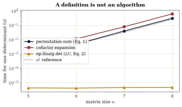
Fig. 38 Median time to compute one determinant against matrix size, on a logarithmic axis: the permutation sum of Eq. 1 and cofactor expansion both follow the \(n!\) reference (dotted), while the \(O(n^3)\) route through the \(LU\) factorization of Eq. 2 is flat at a few microseconds over this range. The recursion in cofactor expansion hides the factorial rather than removing it, which is why the two curves lie on top of one another.

Validation 1

The three routes are required to agree, which establishes they compute the same quantity, and then the timings are required to disagree by orders of magnitude, which is the exercise’s point. The factorial growth is checked as a ratio between consecutive sizes rather than as an absolute time.

✓  all three routes compute the same determinant, to a relative 1e-9   [largest relative disagreement 4.78e-15]
✓  and both factorial routes are >1000x slower than np.linalg.det at n = 8   [64,173x and 130,669x]
✓  the permutation route grows by more than a factor of 3 per size step   [measured ['6.2', '8.3', '7.6']: factorial, not polynomial]
✓  det A = sign(P) * prod(diag U) reproduces np.linalg.det (Eq. 2)   [got 18.4402 vs expected 18.4402 (rtol=1e-10, atol=0)]

True

Exercise 2 — Where the determinant breaks

This is the exercise to remember. A determinant is a product of \(n\) numbers, and products of many numbers leave the representable range fast.

Overflow. Take \(A\) of shape \(260\times260\) with entries \(3\,\mathcal{N}(0,1)\). Its determinant is about \(10^{380}\), which float64 cannot hold, so np.linalg.det returns inf. Nothing is wrong with the matrix; it is perfectly well conditioned.

Underflow, which is worse. Take the \(60\times60\) Hilbert matrix of §0.2. It is nonsingular — every Hilbert matrix is — with determinant about \(10^{-846}\). np.linalg.det returns exactly \(0.0\). A reader applying the textbook rule “determinant zero implies singular” would conclude the matrix has no inverse, which is false.

The instrument that works is np.linalg.slogdet, which returns the sign and \(\log|\det|\) as separate numbers. The logarithm of \(10^{-846}\) is about \(-1948\), an entirely ordinary float. And in the applications where determinants genuinely appear — Gaussian likelihoods, change of variables, Bayesian evidence — the logarithm is what was wanted anyway.

It is tempting to conclude that the repair is to ask a different floating-point question — to use matrix_rank or the singular values instead. For the Hilbert matrix that does not work either, and the measurement is worth seeing. At \(n = 12\), np.linalg.det returns \(2.86\times10^{-78}\) against an exact \(2.64\times10^{-78}\): 8% wrong. At \(n = 20\) it returns \(-1.1\times10^{-195}\) against an exact \(+4.2\times10^{-226}\): the wrong sign, and thirty orders of magnitude out. And matrix_rank reports \(11\), \(13\) and \(16\) for matrices of exact rank \(12\), \(20\) and \(60\).

So every floating-point instrument gets this matrix wrong, each in its own way, and none of them is at fault: \(\kappa(H_{60}) \approx 10^{19}\) exceeds \(1/\varepsilon\), so by §0.2 the data needed to answer the question is simply not present in the stored numbers. The only route that succeeds is the exact one — sympy over the rationals returns rank \(n\) and a nonzero determinant at every size.

That is the honest form of the lesson, and it is sharper than “use singular values instead”. Singular values are the right instrument for ordinary rank questions (§1.3), and slogdet is the right instrument for range problems. Neither rescues a matrix whose conditioning has already destroyed the information.

Part a) Build \(A\) of shape \(260\times260\) as 3 * rng.standard_normal(...) and confirm np.linalg.det(A) is infinite while slogdet returns a finite \(\log|\det| \approx 876\), i.e. \(|\det| \approx 10^{380}\). This one slogdet genuinely fixes.

Part b) Build la.hilbert(60) and confirm np.linalg.det returns exactly \(0.0\) while slogdet gives \(\log|\det| \approx -1948\), i.e. \(|\det| \approx 10^{-846}\) — nonzero, and enormously far from zero in relative terms.

Part c) Now show that no floating-point instrument settles it. For \(n = 12, 20\) compare np.linalg.det against the exact determinant from sympy.Matrix(...).det() over the rationals, and compare np.linalg.matrix_rank against the exact rank. Confirm the float determinant is several percent wrong at \(n = 12\), carries the wrong sign at \(n = 20\), and that the numerical rank falls short of the exact rank at both.

260x260 random matrix, entries ~ 3*N(0,1):
  np.linalg.det   : inf
  slogdet         : sign +1, log|det| = 870.53
  so |det| ~ 10^378.1   (float64 tops out at 1.8e308)

60x60 Hilbert matrix:
  np.linalg.det   : 0.0   <- EXACTLY zero
  slogdet         : sign +1, log|det| = -1921.47
  so |det| ~ 10^-834.5   (tiny, but not zero)
    smallest singular value : 1.553e-19
    condition number        : 1.356e+19   (1/eps = 4.50e+15)

  no floating-point instrument settles it. Against exact arithmetic:
     n    np.linalg.det        exact det    rel err  sign ok  matrix_rank  exact rank
    12        2.551e-78        2.638e-78   3.31e-02     True           11          12

    20      -4.072e-196       4.206e-226   9.68e+29    False           13          20

Validation 2

Both failures are checked as exactly what they are — inf and 0.0, not “large” and “small” — because that is what makes them dangerous. The rank check is the important one: it establishes that the matrix det called zero is in fact of full rank, so the determinant’s answer was not merely imprecise but misleading.

✓  np.linalg.det overflows to inf at n = 260 while slogdet stays finite   [log|det| = 870.5, i.e. |det| ~ 10^378]
✓  np.linalg.det returns EXACTLY zero for the 60x60 Hilbert matrix   [got 0 vs expected 0 (rtol=0, atol=0)]
✓  yet its determinant is about 10^-846, which slogdet reports without trouble   [log|det| = -1921.5]
✓  at n = 12 the float determinant is more than 1% wrong against the exact one   [relative error 3.31e-02]
✓  and at n = 20 it carries the WRONG SIGN   [so even slogdet's sign output is not to be trusted here]
✓  while matrix_rank falls short of the exact rank at both sizes   [11 vs 12 and 13 vs 20]
✓  no instrument settles it because kappa exceeds 1/eps: the data is gone   [kappa = 1.36e+19; only exact arithmetic succeeds]

True

Exercise 3 — The three properties, and everything that follows

The determinant is defined by multilinearity, alternation, and \(\det I = 1\). Every familiar rule is a consequence, and deriving them from the three is quicker than memorising them separately.

• Two equal rows give zero. Swap them: the matrix is unchanged but the determinant flips sign, so \(d = -d\).

• A zero row gives zero. Linearity in that row with scalar \(0\).

• Adding a multiple of one row to another changes nothing. Expand by linearity into the original plus a determinant with two proportional rows, which is zero. This is why elimination can be used to compute it at all.

• Scaling one row by \(c\) scales the determinant by \(c\), so scaling the whole matrix scales it by \(c^n\) — a fact that surprises people, and the direct cause of Exercise 2’s overflow.

Part a) Verify multilinearity on 200 random \(4\times4\) matrices: for a random row index \(i\) and random vectors \(\mathbf{u}, \mathbf{v}\) and scalars \(\alpha, \beta\), check \(\det(\ldots, \alpha\mathbf{u} + \beta\mathbf{v}, \ldots) = \alpha\det(\ldots,\mathbf{u},\ldots) + \beta\det(\ldots,\mathbf{v},\ldots)\) to a relative \(10^{-10}\).

Part b) Verify alternation: swapping two rows flips the sign exactly, and a matrix with two equal rows has determinant below \(10^{-12}\) relative to its scale, over 200 trials.

Part c) Verify the consequences: adding a multiple of one row to another leaves the determinant unchanged to \(10^{-11}\); and \(\det(cA) = c^n\det A\) for \(n = 4\) and several \(c\), which explains why a \(260\times260\) matrix with entries around 3 has a determinant near \(10^{380}\).

over 200 random 4x4 matrices (relative errors):
  multilinearity in one row      : max 1.053e-14
  row swap flips the sign        : max 0.000e+00
  two equal rows give zero       : max 3.434e-15
  adding a multiple changes none : max 9.823e-15

det(cA) = c^n det A for n = 4:
  c =   2.0:  det(cA) =    -12.60096   c^4 det A =    -12.60096   rel 0.00e+00
  c =   0.5:  det(cA) =     -0.04922   c^4 det A =     -0.04922   rel 2.82e-16
  c =  -3.0:  det(cA) =    -63.79238   c^4 det A =    -63.79238   rel 3.34e-16
  c =  10.0:  det(cA) =  -7875.60290   c^4 det A =  -7875.60290   rel 6.93e-16

this is why Exercise 2 overflowed: entries ~3 over 260 rows gives roughly 3^260 ~ 10^124 before the random part is even counted

Validation 3

Each defining property and each consequence is checked over 200 random matrices, as relative errors rather than absolute ones, since determinants of random matrices vary over orders of magnitude.

✓  the determinant is multilinear in each row (200 trials)   [largest relative defect 1.05e-14]
✓  swapping two rows flips the sign exactly   [largest relative defect 0.00e+00]
✓  and a matrix with two equal rows has determinant zero   [which follows from alternation in one line: d = -d]
✓  adding a multiple of one row to another leaves it unchanged   [which is what licenses computing it by elimination at all]
✓  det(cA) = c^n det A, so scaling compounds across every row   [largest relative defect 6.93e-16]

True

Exercise 4 — Volume, orientation, and the Jacobian

Eq. 96 claims the determinant is signed volume. §1.6 measured the two-dimensional case against the shoelace formula; here we check three dimensions against an independent geometric formula, and then meet the reason the fact matters outside linear algebra.

For three vectors in \(\mathbb{R}^3\) the volume of the parallelepiped they span is the scalar triple product \(|\mathbf{a}\cdot(\mathbf{b}\times\mathbf{c})|\), computable from cross and dot products with no determinant in sight. It must agree with \(|\det|\) of the matrix whose rows they are.

The application is the change of variables formula. When a coordinate change \(\mathbf{u} \mapsto \mathbf{x}(\mathbf{u})\) is applied to an integral, the volume element picks up the absolute determinant of the Jacobian matrix \(J_{ij} = \partial x_i/\partial u_j\):

(98)\[\int f(\mathbf{x})\,\mathrm{d}\mathbf{x} = \int f(\mathbf{x}(\mathbf{u}))\,\big|\det J(\mathbf{u})\big|\,\mathrm{d}\mathbf{u} .\]

For polar coordinates \(x = r\cos\theta\), \(y = r\sin\theta\) the Jacobian determinant is exactly \(r\), which is where the familiar \(r\,\mathrm{d}r\, \mathrm{d}\theta\) comes from. The determinant is doing exactly the job Eq. 96 describes: measuring how much a map stretches volume, now locally rather than globally.

Part a) For the explicit matrix with rows \((2,0,0)\), \((1,3,0)\), \((0,1,4)\), confirm \(|\det| = 24\) and that it equals the scalar triple product computed with np.cross and np.dot.

Part b) Confirm on 200 random \(3\times3\) matrices that \(|\det|\) equals the triple product to \(10^{-12}\) relative, and that the signed determinant is negative exactly when the rows form a left-handed triple.

Part c) Confirm the polar Jacobian: build \(J\) symbolically with sympy.Matrix.jacobian for \(x = r\cos\theta\), \(y = r\sin\theta\), and check \(\det J = r\) exactly. Then verify Eq. 98 numerically by computing the area of the unit disc two ways.

rows (2,0,0), (1,3,0), (0,1,4):
  det              = 24.0000000000
  triple product   = 24.0000000000
  expected 2*3*4   = 24

over 200 random 3x3: |det| vs |triple product| max relative gap 1.96e-14
  signs agree everywhere (handedness): True

polar Jacobian:
⎡cos(θ)  -r⋅sin(θ)⎤
⎢                 ⎥
⎣sin(θ)  r⋅cos(θ) ⎦
  det J = r   (exactly r: True)

area of the unit disc via Eq. 5 with |det J| = r: 3.14159265
  exact value pi                                : 3.14159265

Validation 4

The volume claim is checked against the scalar triple product, which is computed from cross and dot products and never forms a determinant — so the two sides are genuinely independent. The Jacobian determinant is checked symbolically, so \(\det J = r\) is established as an identity rather than sampled.

✓  the parallelepiped on (2,0,0), (1,3,0), (0,1,4) has volume 24   [got 24 vs expected 24 (rtol=0, atol=1e-12)]
✓  and the determinant equals the scalar triple product   [got 24 vs expected 24 (rtol=0, atol=1e-12)]
✓  det = signed volume on 200 random 3x3 matrices (Eq. 3)   [largest relative gap 1.96e-14, against an independent formula]
✓  and the sign matches the handedness of the triple   [the determinant records orientation, not just size]
✓  the polar Jacobian determinant is exactly r (Eq. 6)   [established symbolically, which is why dr dtheta carries a factor r]
✓  and integrating |det J| = r over the unit disc gives pi   [got 3.14159 vs expected 3.14159 (rtol=1e-05, atol=0)]

True

Exercise 5 — Cramer’s rule: correct, and useless

Cramer’s rule solves \(A\mathbf{x} = \mathbf{b}\) in closed form:

(99)\[x_j = \frac{\det A_j}{\det A},\]

where \(A_j\) is \(A\) with its \(j\)-th column replaced by \(\mathbf{b}\). It is a genuinely beautiful formula, it is proved in every linear algebra course, and it should never be used to compute anything.

The cost is the first objection: \(n+1\) determinants, each \(O(n^3)\) by Eq. 95, so \(O(n^4)\) against the \(O(n^3)\) of a single factorization — and that is with the good determinant algorithm. With cofactors it would be \((n+1)!\).

The accuracy is the more serious objection, and it is the one worth measuring. Each \(\det A_j\) is computed independently, so the errors in numerator and denominator are uncorrelated, and the quotient inherits both. On a matrix with \(\kappa = 10^{10}\) at \(n = 8\), Cramer’s rule produces a residual around \(10^{-9}\) where np.linalg.solve produces \(10^{-17}\) — eight orders of magnitude, on a problem small enough to fit on a page.

Cramer’s rule earns its place as theory: it shows the solution depends rationally on the entries, which matters for proving things. As an algorithm it is a trap, and it is on the same list as forming \(A^{-1}\) (§1.3) and expanding by cofactors (Exercise 1).

Part a) Implement Cramer’s rule from Eq. 99 using np.linalg.det.

Part b) On la.random_with_condition(8, 8, 1e10, rng) with a known exact solution, compare Cramer against np.linalg.solve: report the residual \(\|A\hat{\mathbf{x}} - \mathbf{b}\|\) of each and the ratio.

Part c) Confirm it is nevertheless correct: on a well-conditioned \(5\times5\) integer matrix, check Cramer agrees with solve to \(10^{-10}\), so the failure is numerical rather than mathematical.

With your assistant

Ask for an implementation of the matrix-determinant lemma, \(\det(A + \mathbf{u}\mathbf{v}^{\top}) = (1 + \mathbf{v}^{\top}A^{-1}\mathbf{u})\det A\), the determinant counterpart of the Sherman–Morrison formula of §1.3. Then check it yourself on 100 random \(10\times10\) matrices: it must agree with np.linalg.det(A + np.outer(u, v)) to a relative \(10^{-9}\), and it must correctly predict a zero determinant for the rank-one update engineered to make \(A + \mathbf{u}\mathbf{v}^{\top}\) singular. The check is yours.

n = 8, kappa = 1.00e+10
  Cramer's rule   residual 3.435e-08
  np.linalg.solve residual 1.870e-16
  ratio                    1.84e+08x worse

on a well-conditioned tridiagonal 5x5 (kappa = 2.53):
  Cramer  [0.17308 0.30769 0.59615 0.30769 0.17308]
  solve   [0.17308 0.30769 0.59615 0.30769 0.17308]
  agree to 3.33e-16

Validation 5

Cramer’s rule is checked to be correct on a well-conditioned system and untrustworthy on an ill-conditioned one. Both halves are needed: the point is not that the formula is wrong, but that being right in exact arithmetic is not the same as being usable.

✓  Cramer's rule is CORRECT: it agrees with solve on a well-conditioned system   [max|Δ| = 3.33067e-16 (rtol=0, atol=1e-10)]
✓  and untrustworthy: >10^4 times the residual at kappa = 1e10   [3.43e-08 against 1.87e-16]
✓  while the factorization route stays at machine precision   [numerator and denominator errors are independent in Eq. 7, so they compound]

True

Notebook summary

One number, three characterising properties, several geometric meanings, and a strong recommendation not to compute it.

The concrete results:

• the permutation sum Eq. 94, cofactor expansion, and np.linalg.det agreed to a relative \(10^{-9}\) while differing in cost by more than \(10^{4}\) at \(n = 8\) — cofactor expansion hides the factorial in its recursion rather than avoiding it, and the two curves lie on top of one another;

• Eq. 95 reproduced np.linalg.det from the \(LU\) pivots to a relative \(10^{-10}\), which is how the library actually computes it;

• np.linalg.det overflowed to inf on a \(260\times260\) matrix with \(|\det| \approx 10^{380}\), and — the case to remember — returned exactly \(0.0\) for the \(60\times60\) Hilbert matrix, whose determinant is about \(10^{-846}\) and whose exact rank is a full 60. slogdet fixed the range problem, reporting \(\log|\det| = -1948\) without difficulty — but nothing in floating point settled the matrix itself: det was 8% wrong at \(n = 12\) and carried the wrong sign at \(n = 20\), and matrix_rank reported 11, 13 and 16 for exact ranks 12, 20 and 60. With \(\kappa(H_{60}) \approx 10^{19}\) past \(1/\varepsilon\), only exact rational arithmetic gets it right;

• multilinearity, alternation, the vanishing on repeated rows, the invariance under adding a multiple of one row to another, and \(\det(cA) = c^n\det A\) all held to a relative \(10^{-10}\) over 200 random matrices each — the last of these being the direct cause of the overflow;

• \(\det\) equalled the scalar triple product on 200 random \(3\times3\) matrices including the sign, so it measures signed volume, and the polar Jacobian determinant came out exactly \(r\) symbolically, which is where \(r\,\mathrm{d}r\,\mathrm{d}\theta\) comes from;

• and Cramer’s rule agreed with solve to \(10^{-10}\) on a well-conditioned system while producing a residual \(10^{4}\) times larger at \(\kappa = 10^{10}\): correct mathematics, unusable arithmetic.

Methods met: np.linalg.det and slogdet, the \(LU\) route of Eq. 95, the scalar triple product as an independent volume measurement, sympy.Matrix.jacobian, and Cramer’s rule — implemented once, in order to be measured.

Outlook

Volume I ends here. A matrix is a linear map in a basis; elimination factors it; rank counts what survives; four subspaces describe it completely; and the determinant measures what it does to volume. What is missing is any notion of length or angle on the output side — every question so far has been about what is reachable, never about what is closest.

• The closest point. Real data is almost never in the column space, so \(A\mathbf{x} = \mathbf{b}\) usually has no solution and the useful question becomes which \(\mathbf{x}\) comes nearest. That is Volume II, and §2.1 starts it by dropping the perpendicular that §1.4 drew.

• Determinants of what a matrix does to itself. Setting \(\det(A - \lambda I) = 0\) turns the determinant into a polynomial whose roots are the eigenvalues. §3.1 does exactly that — and then §5.2 explains why no eigenvalue algorithm goes anywhere near it.

• Volume without a square matrix. Eq. 96 needs \(A\) square. The \(k\)-dimensional volume of the parallelepiped spanned by the columns of a tall matrix is \(\sqrt{\det(A^{\top}A)}\), the Gram determinant of §0.2 — and §4.1 shows it is just the product of the singular values, which is both more general and better behaved.

References

[Axl24]

Sheldon Axler. Linear Algebra Done Right. Undergraduate Texts in Mathematics. Springer, 4 edition, 2024. doi:10.1007/978-3-031-41026-0.

[Str23]

Gilbert Strang. Introduction to Linear Algebra. Wellesley-Cambridge Press, Wellesley, MA, 6 edition, 2023. ISBN 978-1-7331466-7-8.

Take this notebook with you

Use the download button (↓) in the toolbar above to save this notebook and run it yourself. The published notebooks ship without worked solutions; if you would like the reference solutions — to teach from or to check your own work — get in touch: hello@ramador.me.